Firm Objectives, Costs and Revenue
Objectives
Profit maximisation is a useful benchmark because profit rewards entrepreneurship and finances survival, investment and growth. However, ownership and control may be separated, information is imperfect, and firms may pursue several objectives.
| Objective | Meaning | Possible reason |
|---|---|---|
| Profit maximisation | greatest TR−TC | owners’ return and investment finance |
| Profit satisficing | acceptable rather than maximum profit | uncertainty or managerial discretion |
| Revenue maximisation | maximise total sales revenue | growth, status or managerial preference |
| Market-share dominance | increase sales relative to competitors | future market power, network effects or strategic positioning |
| Survival | maintain liquidity and operations | recession or intense competition |
| Social objectives | people/environment alongside finance | mission, reputation or stakeholder pressure |
Why objectives differ
- Information limits: exact demand and cost conditions may be unknown, so a precise maximum cannot be identified in advance.
- Ownership-control separation: managers may value growth, status, job security or organisational slack differently from shareholders.
- Stage and context: a new firm may prioritise survival or market share, while a mature firm may prioritise cash flow or dividends.
- Stakeholders and constraints: lenders, workers, regulators, communities and environmental commitments can constrain the feasible objective.
Revenue maximisation occurs where if there is no binding minimum-profit constraint. Market-share dominance concerns sales volume or relative position, so it is not identical to revenue maximisation. Profit satisficing means achieving an acceptable profit rather than the greatest possible profit, often because information is incomplete or decision-makers pursue several goals.
Economic cost and profit
- Explicit cost: direct monetary payment.
- Implicit cost: opportunity cost of owner-supplied resources.
- Accounting profit: TR minus explicit cost.
- Economic profit: TR minus explicit and implicit cost.
- Normal profit: minimum entrepreneurial return required to remain; included in economic cost.
Worked economic-profit distinction
Suppose a business earns revenue of $240,000, pays explicit costs of $170,000, and uses an owner-managed building that could earn rent of $30,000 elsewhere.
The forgone rent is an implicit opportunity cost. If economic profit were zero, the owner would still be receiving normal profit through the imputed return included in economic cost.
Production periods
- Short run: at least one factor is fixed.
- Long run: all factors are variable.
The distinction depends on adjustability, not clock time. A restaurant may be able to vary staff hours and ingredients this week but not the size of its premises, so it is operating in the short run. Once it can relocate, enlarge the kitchen or choose a different plant, those factors are variable and the decision is long run. The short run can therefore last days in one industry and years in another.
“Fixed” also refers to the factor or cost with respect to current output, not to something that can never change. Rent on the existing premises may be fixed over the present production period even though the firm can renegotiate or move later.
Short-run cost
- Total fixed cost (TFC): cost that does not vary with current output in the short run.
- Total variable cost (TVC): cost that changes with output.
- Total cost (TC): .
- Average fixed, variable and total cost: cost per unit of output.
- Marginal cost (MC): additional total cost from producing one more unit, or for a discrete change.
For positive output :
Total costs are measured over a period, average costs are measured per unit of output, and marginal cost is the change in total cost per additional unit. Keeping these units distinct prevents a common error: MC is not “the total cost of the last unit”; it is the amount by which total cost changes when output changes.
Worked cost link
Suppose output rises from 4 to 5 units. TFC remains $20, while TVC rises from $28 to $35.
| Quantity | TFC | TVC | TC | AFC | AVC | AC |
|---|---|---|---|---|---|---|
| 4 | $20 | $28 | $48 | $5 | $7 | $12 |
| 5 | $20 | $35 | $55 | $4 | $7 | $11 |
The fifth unit adds $7 to variable and total cost, so:
AFC falls because the same fixed cost is divided over more units. AVC happens to remain $7 in this example; neither result implies an economy of scale because the calculation concerns one fixed plant in the short run.
Syllabus boundary
You must understand and use cost and revenue concepts, but the derivation of cost and revenue curves is not required. The explicit functions behind the figures are used to guarantee accurate geometry, not to create an additional derivation requirement.
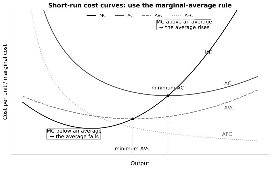
Caption: The horizontal axis is output per period and the vertical axis is cost per unit or per additional unit. AFC falls continuously because a fixed total is spread over more output. AVC and AC are U-shaped in the schematic model. MC crosses each average at its minimum: when MC lies below an average it pulls that average down, and when MC lies above it, it pulls the average up. AC remains above AVC because . Deriving the exact curves is enrichment; interpreting these relationships is core.
MC cuts AVC and AC at their minima:
- MC below average → average falls;
- MC above average → average rises.
AFC never determines MC because fixed cost does not change when one more unit is produced.
The marginal-average rule is the same logic as a class average. A new score below the existing average lowers it; a new score above the average raises it. MC is the cost of the additional output, so it changes AVC or AC in the same direction. This explains the intersections rather than requiring their positions to be memorised.
Why marginal cost eventually rises
With at least one fixed factor, adding units of a variable factor eventually causes diminishing marginal returns: marginal product falls because the fixed factor becomes increasingly congested or overused.
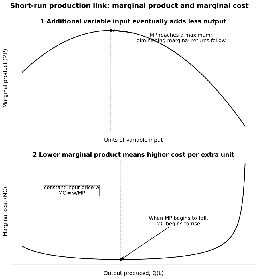
Caption: The top panel measures the extra output produced by another unit of the variable input; the bottom panel measures the cost of another unit of output. With a constant price for the variable input, . Rising MP initially lowers MC, while diminishing marginal returns make MP fall and MC rise. The vertical guide marks the turning region; it is not a long-run scale effect. This diagram is explanatory enrichment.
This is a short-run production explanation, not an economies-of-scale explanation. Economies of scale concern changes in all inputs in the long run.
Revenue
- Total revenue (TR): the firm’s receipts from sales, equal to price multiplied by quantity when all units are sold at the stated price.
- Average revenue (AR): revenue per unit sold; it equals price when every unit is sold at the same price.
- Marginal revenue (MR): the change in total revenue caused by selling one additional unit, or for a discrete change.
AR is normally the price received per unit. For a price taker, selling another unit does not change market price, so . For a price setter facing downward-sloping demand, selling more normally requires a lower price; MR lies below AR because the lower price applies not only to the extra unit but also to earlier units.
The AR curve is also the demand curve facing the firm because, at each quantity, it records the price buyers are willing to pay per unit. This is not always the same as market demand. In perfect competition the individual firm is too small to affect the market price, so its own demand is horizontal at the market price even though market demand slopes downward.
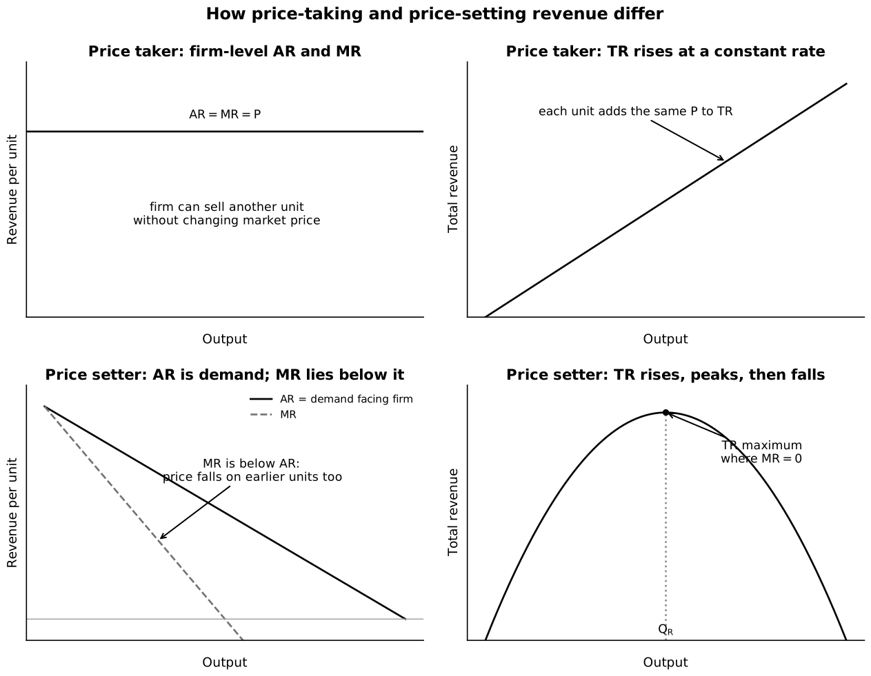
Caption: The upper panels show a price taker: horizontal means every extra unit adds the unchanged market price to TR, so TR rises linearly. The lower panels show a price setter: AR is the firm’s downward-sloping demand curve, MR lies below AR because selling more requires a price reduction on earlier units, and TR reaches its maximum where . These are firm-level curves; the horizontal price-taking AR is not the market demand curve.
Worked revenue calculation
Suppose a price-setting firm sells 4 units at $12 each and must lower price to $10 to sell 5 units.
Although the fifth unit sells for $10, marginal revenue is only $2 because lowering price reduces revenue earned on the first four units.
Profit versus sales-revenue maximisation
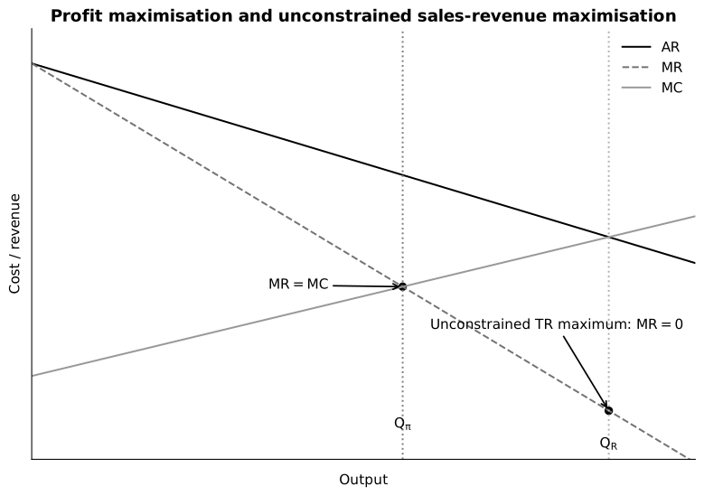
Caption: A profit maximiser chooses output where with MC rising through MR, while a sales-revenue maximiser expands output until , provided financial survival or a minimum-profit constraint is satisfied.
In the standard case shown—downward-sloping demand, declining MR over the relevant range and positive MC—the sales-revenue-maximising output exceeds the profit-maximising output. It therefore involves a lower price. Treat this as a result of the stated conditions, not an unconditional rule for every possible cost and demand function.
Decision quality under uncertainty
An objective is not enough to guarantee an optimal decision. Firms may forecast demand incorrectly, misestimate competitors’ reactions, overlook implicit costs, or continue a failing project because of sunk costs already incurred. Good analysis therefore separates:
- the objective being pursued;
- the information and constraints available;
- the decision rule used;
- the realised outcome, which may differ from the intended outcome.
Common pitfalls
- Counting the owner’s forgone salary as explicit cost.
- Calling normal profit a supernormal reward.
- Attributing falling AFC to economies of scale; AFC is a short-run spreading effect.
- Using diminishing marginal returns to explain the long-run LRAC.
- Assuming AR always slopes downward.
- Saying revenue is maximised where AR=0 rather than MR=0.
- Confusing marginal cost with average cost of the final unit.
Return to Firms and Decisions.