Profit Maximisation and Firm Equilibrium

Marginal rule

Profit changes by:

$$\text{marginal profit}=MR-MC$$

• $MR>MC$: another unit raises profit.
• $MR<MC$: another unit lowers profit.
• Maximum profit occurs where $MR=MC$ and MC is rising through MR.

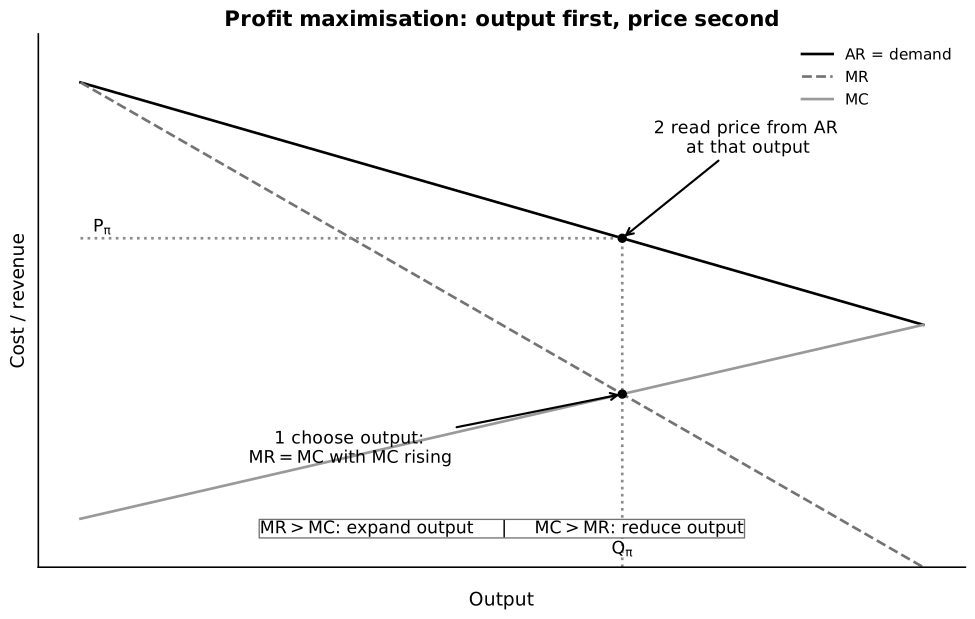
Caption: The horizontal axis is firm output and the vertical axis is revenue or cost per unit. Output $Q_{\pi }$ is chosen where rising MC crosses MR because units before it add more revenue than cost and units after it add more cost than revenue. For a price setter, move vertically from $Q_{\pi }$ to AR—the demand curve facing the firm—to read $P_{\pi }$. The lower MR=MC coordinate is not the selling price.

Do not choose price at the vertical coordinate of MR=MC.

Profit outcomes

$$\text{economic profit}=(AR-AC)\times Q$$

This formula follows from totals:

$$\pi =TR-TC=(AR\times Q)-(AC\times Q)=(AR-AC)Q.$$

At the chosen output, $AR-AC$ is profit per unit. Multiplying that vertical gap by the number of units gives the rectangular area of total profit. If $AR<AC$, the gap is negative and the corresponding rectangle represents total economic loss—not deadweight loss.

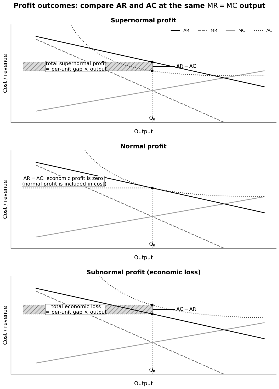
Caption: Each panel first chooses output where rising MC crosses MR and then compares AR with AC at that same quantity. If AR exceeds AC, the vertical gap times output is supernormal profit; if AR equals AC, economic profit is zero and the firm earns normal profit; if AR is below AC, the vertical loss per unit times output is subnormal profit. The shaded rectangle is a private profit or loss area, not a social-welfare triangle.

Normal profit means economic profit is zero, not that the owner receives nothing.

Profit maximisation versus revenue maximisation

A profit maximiser stops expanding when $MR=MC$. An unconstrained sales-revenue maximiser continues until $MR=0$, because TR rises while MR is positive and falls after MR becomes negative. With positive MC and the standard downward-sloping demand shown in the topic figure, the revenue-maximising output is therefore larger and its price lower. A real firm may require a minimum profit, so the attainable revenue-maximising output can lie before the unconstrained $MR=0$ point.

Shutdown

In the short run, fixed cost is unavoidable.

Syllabus boundary

The shutdown condition is required, but diagrammatic shutdown analysis is not. Use the figure as enrichment to understand the rule; in an examination, prioritise the verbal or numerical comparison requested.

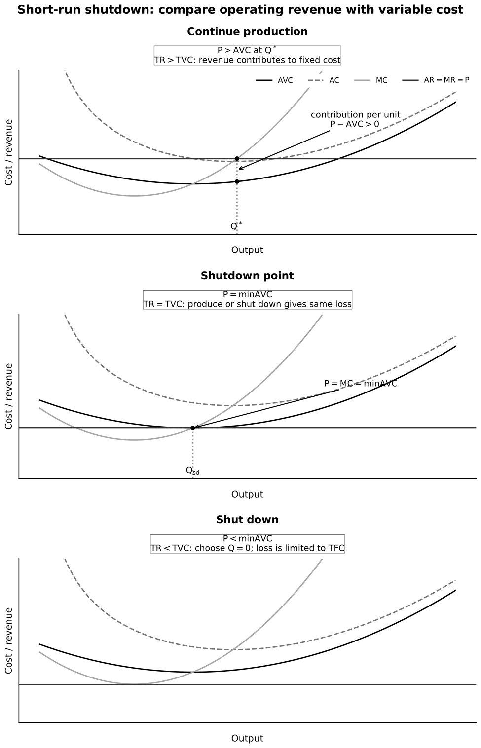
Caption: In each price-taking panel, the horizontal AR=MR line is market price and the firm would produce where it meets rising MC. Compare price with AVC at that output. Above AVC, operating revenue covers all variable cost and contributes toward fixed cost; at minimum AVC the firm is indifferent; below AVC, operating adds an uncovered variable-cost loss, so zero output minimises short-run loss. The diagram is explanatory enrichment; the verbal $TR$–$TVC$ rule is core.

• $AR>AVC$: continue; variable cost and part or all of fixed cost are covered.
• $AR=AVC$: indifferent between producing and shutting down in the short run.
• $AR<AVC$: shut down; producing would not cover variable cost and would increase loss.

Equivalently, compare totals: continue when $TR\ge TVC$ and shut down when $TR<TVC$. A loss-making firm may therefore continue in the short run if operating reduces its loss relative to paying all fixed cost with zero output.

Worked shutdown comparison

Suppose producing gives revenue of $80, variable cost of $60 and unavoidable fixed cost of $50.

• If the firm produces, $TC=60+50=110$, so its loss is $30.
• If it shuts down, revenue and variable cost are zero but it still pays $50 fixed cost, so its loss is $50.

Producing is rational because the $20 contribution, $TR-TVC$, covers part of fixed cost and reduces loss. If TVC were $90, producing would create a $60 loss, so shutdown would instead limit loss to $50.

Shutdown is temporary cessation. Exit is a long-run departure from the industry.

In the long run no input is fixed, so the firm can avoid future operating costs by leaving the industry. Sunk costs already incurred remain unrecoverable and should not affect the current exit decision. A firm exits if it expects $TR<TC$, equivalently $AR<AC$, to persist when all relevant future opportunity costs are counted.

Long-run adjustment

Syllabus boundary

The economic ideas of entry, exit and long-run adjustment remain useful, but diagrammatic short-run-to-long-run firm adjustment is explicitly not required by 9570.

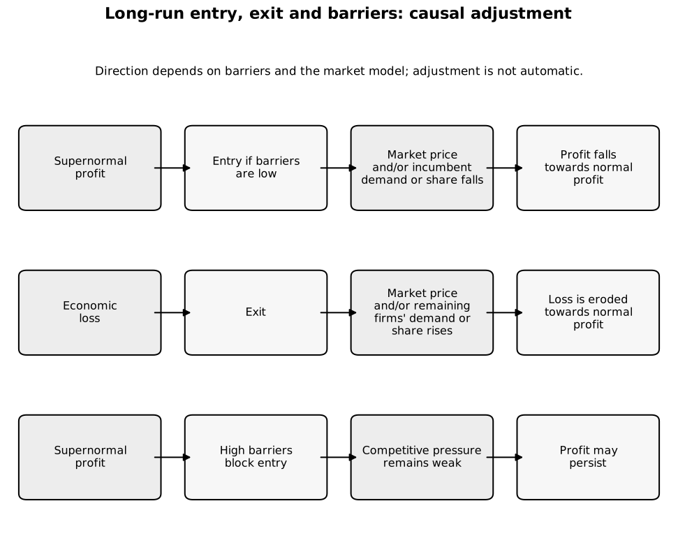
Caption: Read each row from left to right. With low barriers, supernormal profit attracts entry and competitive pressure erodes incumbent profit toward normal; persistent loss causes exit and can improve the demand, price or market share available to survivors. With high barriers, entry is blocked and supernormal profit may persist. The exact adjustment channel differs across market models, so the arrows show conditional causal logic rather than an automatic curve shift.

In perfect competition, entry increases market supply and lowers market price, so the individual firm’s horizontal $AR=MR$ line shifts downward until only normal profit remains. In monopolistic competition, entry divides market demand among more differentiated firms, shifting an incumbent’s demand left (and typically making it more price-elastic) until normal profit remains. Exit reverses the relevant adjustment. Monopoly and oligopoly can retain supernormal profit if barriers persist.

Price-setting versus price-taking

For a price-taking firm, $AR=MR=\text{market price}$. For a price setter, AR slopes downward and MR is below AR.

The same MR=MC rule applies, but the price and long-run adjustment differ.

Step-by-step diagram method

For a price-setting firm:

1. identify the output where rising MC crosses MR;
2. project vertically to AR to obtain the maximum price consumers will pay for that output;
3. compare AR with AC at the same output;
4. calculate profit as $(AR-AC)\times Q$;
5. distinguish the short-run outcome from later entry, exit or strategic response.

For a price taker, market price determines the horizontal AR=MR line. The firm chooses its own output where rising MC crosses that line. The market determines price; the firm does not select both price and output independently.

Why the marginal rule works

Before the optimum, each additional unit adds more revenue than cost, so producing it increases total profit. Beyond the optimum, additional cost exceeds additional revenue. The equality is therefore necessary only at the correct crossing; a falling-MC crossing can mark a minimum or unstable point rather than maximum profit.

Worked marginal decision

Suppose a price-setting firm has:

$$AR=20-Q,MR=20-2Q,MC=4+Q.$$

Profit maximisation requires:

$$20-2Q=4+Q\Rightarrow Q^{\ast }=\frac{16}{3}\approx \mathrm{5.33.}$$

Price is read from AR, not MR or MC:

$$P^{\ast }=20-\frac{16}{3}=\frac{44}{3}\approx \mathrm{14.67.}$$

If $AC=10$ at this output, economic profit is:

$$(14.67-10)(5.33)\approx \mathrm{24.9.}$$

The calculation separates three steps: choose output using $MR=MC$, read price from AR, then compare AR with AC to determine profit.

Common pitfalls

• Saying profit is maximised wherever MR=MC without checking the crossing.
• Reading price from MC or MR.
• Measuring profit using $(P-MC)\times Q$.
• Shutting down whenever economic profit is negative.
• Confusing short-run shutdown with long-run exit.
• Showing entry on a firm diagram without explaining the demand effect.

Return to Firms and Decisions.