Aggregate Supply and AD-AS Equilibrium

Definition and axes

Aggregate supply (AS) is the total real output that firms throughout the economy are willing and able to produce at each general price level (GPL), over a given period.

The horizontal axis is real national output or income; the vertical axis is the GPL. A movement along AS is caused by a GPL change under the curve’s stated assumptions. A change in a non-price determinant shifts AS.

Like AD, AS is a conditional schedule rather than a time path. It asks how much real output firms across the economy are willing and able to produce at each hypothetical GPL, holding the relevant cost and capacity determinants constant.

The Keynesian AS ranges

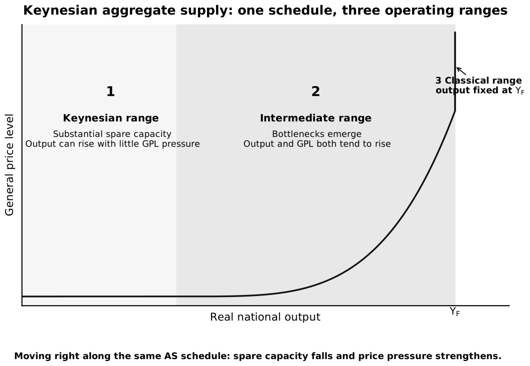
Caption: This is one economy-wide AS curve read from left to right. With substantial spare capacity, additional production uses idle workers and machines with little pressure on unit cost; in the intermediate range, bottlenecks, overtime and less-suitable resources make extra output increasingly costly; at $Y_F$, current resources and technology set a vertical capacity boundary. The ranges explain why the same AD increase can have different output and GPL effects.

Relatively flat Keynesian range

Many workers and machines are idle. Firms can expand production without bidding strongly against one another for scarce inputs, so a rise in AD mainly increases real output and employment with little GPL pressure.

The perfectly horizontal segment is a simplifying limiting case. In reality, some prices may begin rising before all economy-wide spare capacity is exhausted.

Upward-sloping intermediate range

As the economy approaches capacity:

• bottlenecks appear unevenly across sectors;
• firms use less suitable or less productive resources;
• overtime and competition for inputs raise marginal and unit costs.

Firms therefore require a higher GPL to supply additional real output. Both output and GPL respond to an AD change.

Vertical classical range

At full-capacity output, available resources and technology cannot produce more within the relevant horizon. A further AD increase raises the GPL rather than real output.

Full-capacity output is a model boundary. It does not imply that every person is employed, because frictional and structural unemployment can remain.

Short-run costs and long-run capacity

JC materials may use either a single J-shaped Keynesian AS curve or separate SRAS and LRAS curves. State which convention you are using and keep its logic consistent.

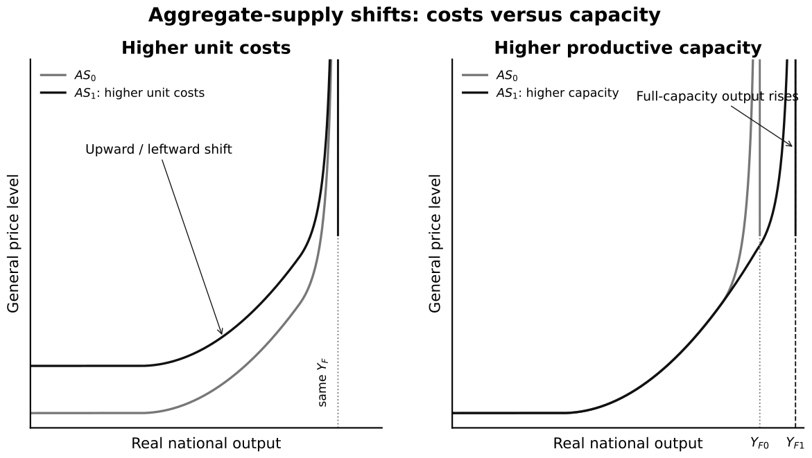
Caption: The left panel holds productive capacity fixed: a higher unit cost means firms supply less output at every GPL, so SRAS shifts upward or left. The right panel changes what the economy can sustainably produce: more or better resources, capital, technology or institutions shift the capacity boundary right. A productivity improvement can do both—lower current unit cost and raise potential output—so the time horizon must be stated.

Cost shift or capacity shift? Use this test

Question	Short-run cost effect	Productive-capacity effect
What changes?	cost per unit at existing capacity	maximum sustainable output
Typical cause	oil price, money wage relative to productivity, indirect business tax	labour quantity/quality, net capital formation, technology, infrastructure
Diagram	SRAS or the rising portion of AS shifts	LRAS or the vertical capacity boundary shifts
Can both occur?	yes	productivity or supply-side investment may lower unit cost now and expand capacity later

SRAS determinants

SRAS changes when economy-wide unit production costs change while productive capacity is given. Examples include:

• money wages relative to labour productivity;
• energy, imported input and raw-material prices;
• indirect business taxes, subsidies and grants;
• short-run supply disruptions and weather shocks;
• expected inflation when it affects wage and price setting.

A rise in unit costs shifts SRAS upward or left: at each GPL, firms supply less real output. A fall in unit costs shifts it downward or right.

Productive-capacity or LRAS determinants

Capacity changes with:

• labour-force size, participation and human capital;
• the capital stock, which rises through net investment;
• the quantity or accessibility of land and natural resources;
• technology, research, innovation and management quality;
• infrastructure and institutions that affect economy-wide productivity.

An increase in capacity shifts the full-employment output boundary or LRAS right. A technology or productivity improvement can affect both horizons: it may lower current unit costs and expand potential output.

Gross investment does not always expand capacity because part of it merely replaces depreciation. Net investment is the relevant addition to the capital stock.

AD-AS equilibrium and adjustment

At the intersection of AD and AS, planned real expenditure equals planned real output at the equilibrium GPL.

If planned expenditure exceeds output at the prevailing GPL, firms experience unintended inventory depletion. They expand production and may raise prices. If planned output exceeds expenditure, inventories accumulate; firms reduce production and may lower the rate of price increase or prices. The strength and speed of price adjustment depend on wage and price flexibility.

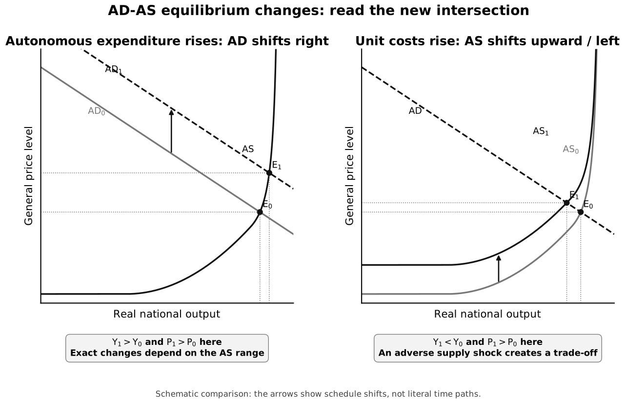
Caption: In the demand panel, AD shifts right while AS is unchanged; locate the new intersection and read both the higher real output and higher GPL. In the adverse-supply panel, AS shifts left while AD is unchanged; the new intersection combines lower real output with a higher GPL. The arrows indicate schedule shifts; the marked $E_0$ and $E_1$ points and dotted guides compare equilibrium coordinates. This is comparative statics, not a claim that the economy literally travels along a fixed time path.

Analysing shocks

Use the same sequence for every shock: identify the determinant, name the curve and direction, explain the schedule change at every GPL, locate the new intersection, read both axes, then qualify by spare capacity and time.

Positive demand shock

For improved consumer confidence:

1. autonomous consumption rises;
2. AD shifts right;
3. inventories fall unexpectedly;
4. firms expand output and factor employment;
5. factor income and induced consumption rise through the multiplier;
6. equilibrium real output and GPL rise;
7. the output gain is larger, and price pressure smaller, when spare capacity is greater.

Adverse short-run supply shock

For a rise in imported energy prices:

1. firms’ unit production costs rise across many sectors;
2. SRAS shifts upward or left;
3. equilibrium real output falls while GPL rises;
4. employment tends to fall as production contracts.

This combination differs from demand-pull inflation. A contractionary demand policy may reduce the GPL pressure but deepen the output loss.

Positive capacity shock

For sustained productivity-enhancing investment:

1. the effective capital stock or technology improves;
2. productive capacity shifts right;
3. the economy can sustain greater real output;
4. at a given AD, the GPL tends to be lower than otherwise;
5. the actual output gain still requires sufficient demand and time for resources to be deployed.

Comparing three common shocks

Shock	Initial curve effect	Real-output effect	GPL effect	Central qualification
confidence raises autonomous $C$	AD right	rises	usually rises	output response is larger with more spare capacity
imported energy becomes dearer	SRAS/AS left	falls	rises	AD may also weaken if real purchasing power falls
productivity-enhancing investment	AD right initially; capacity right later	tends to rise	ambiguous over time	demand pressure may raise GPL first, while later supply expansion reduces it relative to otherwise

Starting position and simultaneous shifts

The same AD shift has different effects along different AS ranges. Moreover, real events can shift both curves. Investment can raise AD immediately and productive capacity later; an imported-energy shock can reduce SRAS while also lowering household real purchasing power and AD. If both curves move, the effect on one axis may be ambiguous and must be analysed conditionally.

Enrichment: classical and Keynesian adjustment

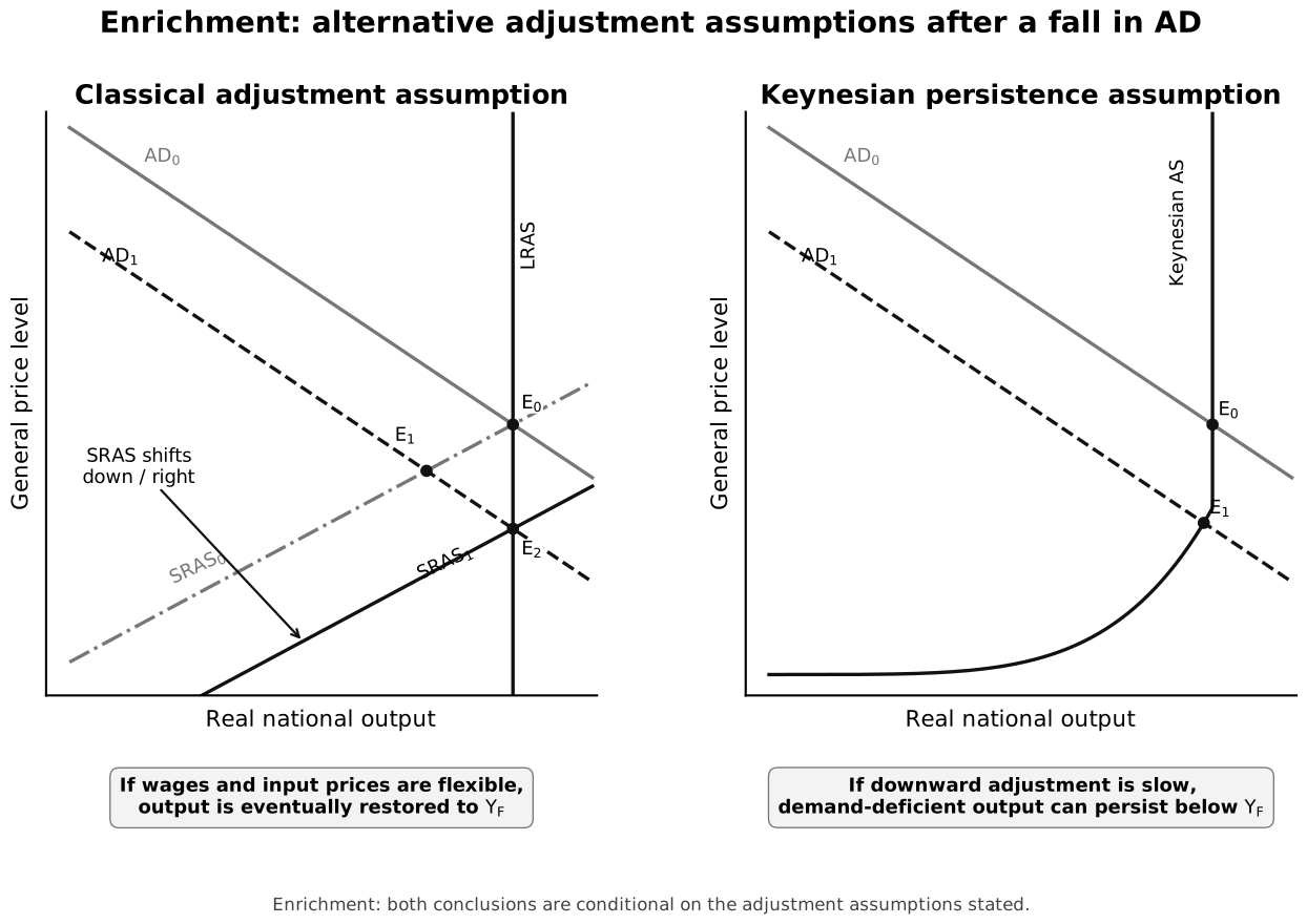
Caption: Both panels begin with a fall in AD. The classical panel assumes sufficiently flexible wages and input prices to lower production costs and shift supply until full-employment output is restored at a lower GPL. The Keynesian panel allows wages, prices and expectations to adjust slowly, so deficient demand and unemployment can persist. This is enrichment: use the contrast to expose assumptions, not as a compulsory school-label diagram.

This contrast is useful background rather than a licence to attach a school label to every conclusion. Always state the operative assumptions: spare capacity, wage-price flexibility, expectations and time horizon.

Common pitfalls

• Labelling the vertical axis “price” rather than GPL.
• Treating a movement up AS as an increase in AS.
• Shifting LRAS for a temporary input-cost rise.
• Assuming every technological improvement affects only LRAS.
• Saying gross investment necessarily expands the capital stock.
• Equating full-capacity output with zero unemployment.
• Claiming an AD increase always raises real output by the same amount.
• Ignoring that a shock can move both AD and AS over different horizons.

Return to Introduction to Macroeconomics.