Circular Flow and National-Income Equilibrium

What the model represents

The circular flow is an interactive model of flows per period among households, firms, government and the foreign sector. It connects:

• real flows of factor services and final output;
• money flows of factor income and expenditure;
• withdrawals from, and injections into, demand for domestic output.

Income is a flow, such as dollars per year. Wealth, inventories and the capital stock are stocks measured at a point in time.

Two-sector closed economy

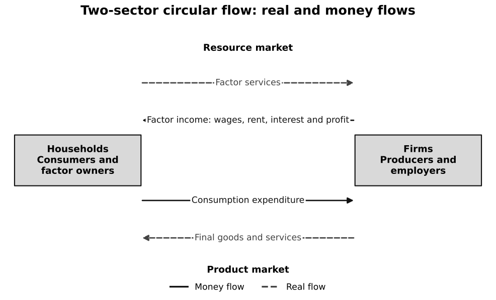
Caption: The upper pair of arrows is the resource market: factor services flow from households to firms, while rent, wages, interest and profit flow back as factor income. The lower pair is the product market: final goods and services flow from firms to households, while consumption expenditure flows back to firms. Every real flow has an opposite money flow, and every arrow is measured per period.

Households are both consumers and owners of factors of production. Firms are both producers and purchasers of factor services. Every market exchange has a real flow and an opposite money flow.

For example, when a household member works for a bakery, labour services flow to the firm and wages flow to the household. When the household buys bread, final output flows back to the household and consumption expenditure flows to the firm. The same production activity therefore creates output, income and expenditure around one circuit.

The same production can be measured by:

1. the value of final output produced;
2. the factor income generated in production;
3. expenditure on that final output.

Hence, after consistent valuation:

$$\text{output}\equiv \text{income}\equiv \text{expenditure}$$

The symbol $\equiv$ marks an accounting identity. It does not mean that firms’ planned output must equal buyers’ planned expenditure before inventories adjust.

Four-sector open economy

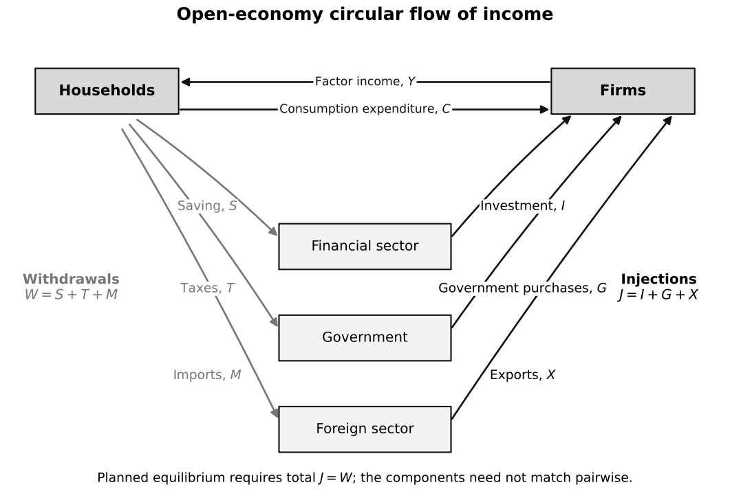
Caption: Begin with household income and trace where it goes. Consumption returns directly to domestic firms; saving, taxes and import expenditure are withdrawals because they do not currently purchase domestic output. Investment, government purchases and exports are injections because they create spending on domestic output from outside the immediate consumption-income loop. The sector boxes show possible channels, not pairwise equalities between $S$ and $I$, $T$ and $G$, or $M$ and $X$.

Withdrawals

$$W=S+T+M$$

• Saving ($S$): current income not spent on consumption. Financial institutions can channel saving toward borrowers, but saving itself is still a withdrawal from current expenditure.
• Taxes ($T$): reduce private disposable income or spending power; the simplified model groups relevant tax flows together.
• Imports ($M$): expenditure on foreign-produced output rather than domestic output.

Injections

$$J=I+G+X$$

• Investment ($I$): expenditure on newly produced capital goods, new residential structures and additions to inventories. Purchases of existing financial assets are not current production and do not count as $I$.
• Government expenditure ($G$): government purchases of currently produced goods and services. Transfer payments are not direct purchases of output.
• Exports ($X$): foreign expenditure on domestically produced goods and services.

The model requires equality of the totals, not pairwise equality: equilibrium does not require $S=I$, $T=G$ or $M=X$ separately.

Withdrawals do not mean money vanishes

“Withdrawal” describes a withdrawal from current expenditure on domestic output, not physical destruction of money.

• Saving may be channelled through financial institutions to firms, but planned investment depends on firms’ borrowing and capital-spending decisions; saving and investment are different decisions.
• Taxes finance government activity, but taxes and government purchases need not be equal in the period because the government can run a budget deficit or surplus.
• Import expenditure becomes income abroad, while export revenue comes from foreign expenditure; the trade balance need not be zero.

This is why only $S+T+M=I+G+X$ is required at planned equilibrium.

Accounting identity versus planned equilibrium

Using the expenditure approach:

$$Y\equiv C+I+G+(X-M)$$

Realised investment includes unintended inventory accumulation or depletion. This makes the accounting identity hold ex post even when firms’ plans were disappointed.

The behavioural equilibrium condition is different:

$$J=W$$

It compares planned injections and withdrawals. If planned $J\ne W$, firms receive an inventory signal and adjust output and employment.

Statement	Type	Why it matters
$Y\equiv C+I+G+(X-M)$	accounting identity	realised inventory investment makes recorded expenditure equal recorded output ex post
$J=W$	behavioural equilibrium condition	planned expenditure is compatible with planned output, so there is no inventory-induced tendency for income to change
$J>W\Rightarrow Y$ tends to rise	adjustment mechanism	unintended inventory depletion encourages more production, employment and factor income

Adjustment toward equilibrium

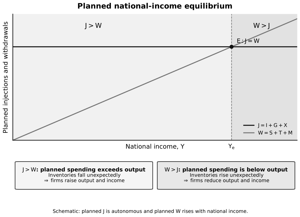
Caption: The horizontal $J$ schedule assumes planned injections are autonomous with respect to current national income. The upward-sloping $W$ schedule shows that saving, tax payments and imports rise as income rises. Their intersection gives equilibrium $Y_e$. Left of $Y_e$, $J>W$ and inventories tend to fall; right of $Y_e$, $W>J$ and inventories tend to accumulate, so output moves back toward the intersection.

When $J>W$

1. planned expenditure on domestic output exceeds current planned production;
2. inventories fall unexpectedly;
3. firms expand output and hire more factors;
4. factor income and induced consumption rise;
5. higher income also raises saving, tax payments and imports;
6. adjustment ends when withdrawals have risen enough to match injections.

When $W>J$

1. planned expenditure is insufficient to purchase current planned output;
2. inventories accumulate unexpectedly;
3. firms cut production and factor employment;
4. income and induced consumption fall;
5. saving, tax payments and imports fall with income;
6. a lower equilibrium income is reached when $W=J$.

The equilibrium can contain unemployment and spare capacity. It means only that there is no current tendency for national income to change.

Worked adjustment

Suppose autonomous planned injections are $80 billion and planned withdrawals are initially $70 billion. The $10 billion gap is not the final rise in income. It first causes unintended inventory depletion. As firms expand production, the additional income generates induced consumption and withdrawals over repeated rounds. Income stops rising only when the cumulative induced increase in $S+T+M$ is $10 billion.

If the marginal propensity to withdraw is $0.4$, the simplified multiplier predicts:

$$\Delta Y=\frac{10}{0.4}=25\text{ billion}$$

The numerical result assumes sufficient spare capacity and no offsetting change in prices or autonomous spending.

Paradox of thrift

Saving is valuable because it can finance investment and future consumption. The paradox of thrift concerns a short-run coordination problem, not a claim that saving is always harmful.

If all households try to save more by cutting consumption while planned investment does not rise, planned withdrawals exceed injections. Firms face unwanted inventories and reduce output and income. Because actual saving depends partly on income, total realised saving may rise by less than households intended, remain unchanged or even fall. The outcome depends on investment responses, financial intermediation, spare capacity and time.

Common pitfalls

• Describing imports as a withdrawal merely because money crosses a border; the key point is that expenditure is not on domestic output.
• Treating saving as money that disappears rather than distinguishing saving from investment.
• Assuming $S=I$, $T=G$ and $M=X$ separately.
• Treating planned and realised investment as identical during disequilibrium.
• Calling purchases of existing shares or second-hand assets current investment.
• Assuming $J=W$ means full employment or an optimal economy.
• Saying income rises immediately by exactly the initial $J-W$ gap.

Return to Introduction to Macroeconomics.