Multiplier Process and Applications

Meaning of the multiplier

The multiplier is the numerical coefficient relating the eventual change in equilibrium national income to the initial autonomous change in planned expenditure on domestic output that caused it:

$$k=\frac{\Delta Y}{\Delta A}$$

Here, $\Delta A$ may come from autonomous consumption, investment, government purchases or net exports. For example, an autonomous rise in exports is positive, while an autonomous rise in imports that substitutes away from domestic output is negative. The multiplier is a process of induced spending, not repeated autonomous government expenditure.

Keep three ideas distinct:

• the multiplier coefficient $k$ is a ratio;
• the multiplier process is the sequence of income, induced domestic consumption and withdrawals;
• the multiplied outcome is the eventual $\Delta Y=k\Delta A$ predicted under the model assumptions.

How the process works

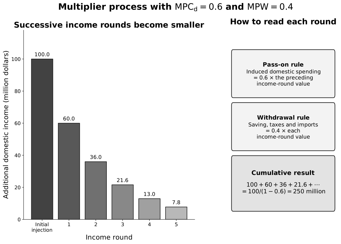
Caption: The first bar is the one-off autonomous injection. Each later bar is induced expenditure on domestic output, equal here to $0.6$ of the preceding income round. The missing $0.4$ of each round is withdrawn through saving, taxes and imports. The bars shrink toward zero; their sum, rather than the height of the final bar, is the total change in equilibrium income.

Suppose autonomous investment rises by $100 million and the marginal propensity to consume domestically produced output is $0.6$:

1. firms receiving the initial $100 million expand output and pay $100 million in factor income;
2. households spend $60 million on domestic consumption and withdraw $40 million through saving, taxes and imports;
3. the $60 million becomes a second round of domestic income;
4. households spend $36 million in the third round;
5. the sequence continues, with each round equal to $0.6$ of the previous round.

Thus:

$$\Delta Y=100+60+36+21.6+\cdots$$ $$\Delta Y=\frac{100}{1-0.6}=250\text{ million}$$

and $k=2.5$.

The process converges because each round is smaller. Cumulative additional withdrawals eventually equal the initial autonomous injection.

The first rounds can be organised as follows:

Income created in round (million dollars)	Induced domestic spending passed to next round (million dollars)	Additional withdrawal in round (million dollars)	Cumulative additional income (million dollars)	Cumulative withdrawals (million dollars)
100.0	60.0	40.0	100.0	40.0
60.0	36.0	24.0	160.0	64.0
36.0	21.6	14.4	196.0	78.4
21.6	13.0	8.6	217.6	87.0

As the sequence continues, cumulative income approaches $250 million and cumulative withdrawals approach the original $100 million injection. The process stops conceptually when the additional injection has been fully matched by additional withdrawals—not because agents literally stop spending.

Marginal propensities and formulas

Marginal propensities measure the response to an additional unit of income. In the simplified four-sector model, define all of them relative to the same $\Delta Y$:

$$MPS=\frac{\Delta S}{\Delta Y},MPT=\frac{\Delta T}{\Delta Y},MPM=\frac{\Delta M}{\Delta Y}$$ $$MPW=MPS+MPT+MPM$$

If $MP{C}_d$ is the marginal propensity to consume domestically produced output:

$$MP{C}_d+MPW=1$$

Therefore:

$$k=\frac{1}{MPW}=\frac{1}{MPS+MPT+MPM}=\frac{1}{1-MP{C}_d}$$

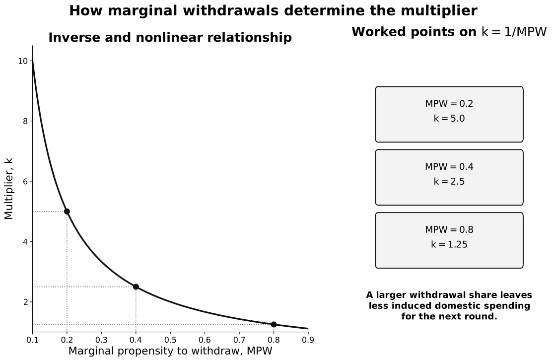
Caption: The horizontal axis is the marginal propensity to withdraw and the vertical axis is $k=1/MPW$. Moving right means a larger share of each additional income round is saved, taxed or spent on imports, so less induced domestic spending reaches the next round and the multiplier falls. The curve is nonlinear: reducing an already small MPW changes $k$ especially strongly.

For a closed economy without proportional taxation:

$$k=\frac{1}{1-MPC}=\frac{1}{MPS}$$

Do not add propensities measured from different income bases. Also do not use an MPC that already includes imported consumption and then subtract imports again through MPM.

For example, an MPC measured from disposable income cannot simply be added to an MPT measured from national income. Either convert the responses to a common $\Delta Y$ denominator or use a formula whose definitions match the data supplied.

Deriving the simple formula

Start from the change in equilibrium expenditure under fixed prices:

$$\Delta Y=\Delta A+MP{C}_d\Delta Y$$

Rearranging:

$$(1-MP{C}_d)\Delta Y=\Delta A$$

Therefore:

$$\frac{\Delta Y}{\Delta A}=\frac{1}{1-MP{C}_d}=k$$

This derivation assumes the induced response is proportional and stable over the relevant income change.

Worked open-economy example

Suppose:

$$MPS=0.20,MPT=0.15,MPM=0.25$$

Then:

$$MPW=0.60,k=\frac{1}{0.60}\approx 1.67$$

An autonomous $300 million export increase gives a fixed-price equilibrium-income change of:

$$\Delta Y=\frac{300}{0.60}=500\text{ million}$$

This is a model prediction, not a guarantee that real output rises by exactly $500 million. If AS is steep, part of the nominal spending increase becomes a higher GPL.

Transfers require an extra step

A transfer payment is not itself $G$ because it does not directly purchase current output. If government transfers an additional $100 million and recipients spend $0.8$ of it on domestic output, the initial autonomous consumption injection is at most:

$$0.8(100)=80\text{ million}$$

The relevant expenditure multiplier is then applied to the $80 million, subject to timing, targeting and other behavioural responses.

It is “at most” $80 million because recipients might repay debt, save abroad, purchase imports or alter other planned spending. Only the net autonomous increase in expenditure on domestic output begins the domestic multiplier process.

Reverse multiplier

A fall in autonomous planned expenditure on domestic output - for example, lower autonomous $C$, $I$, $G$ or $X$, or substitution toward autonomous imports - works through the same mechanism in reverse:

1. AD and firms’ sales fall;
2. inventories accumulate unexpectedly;
3. firms reduce output, employment and factor income;
4. lower income causes induced domestic consumption to fall;
5. successive contractions become smaller because saving, taxes and imports also fall;
6. a lower equilibrium income is reached.

The arithmetic sign changes, but the multiplier coefficient remains positive: a negative $\Delta A$ produces a negative $\Delta Y$.

Assumptions and limitations

The full real-output multiplier requires strong simplifying conditions:

• sufficient spare capacity so firms can expand production;
• a stable GPL or a sufficiently flat AS range;
• stable marginal propensities over the adjustment;
• no offsetting autonomous changes in consumption, investment, government spending or exports;
• no strong crowding-out through interest rates or exchange rates;
• technology and productive capacity given during the short-run process;
• firms respond to sales by changing output rather than only prices;
• enough time for repeated rounds to occur.

In a highly open economy, a large MPM can make $k$ small because induced demand leaks into imports. High marginal saving or taxation also reduces $k$. However, the size of the multiplier is empirical and context-dependent; it should not be inferred from openness alone without evidence.

Near full employment, the formula may still describe an increase in nominal expenditure, but the increase in real output is dampened as the GPL rises. Policy reactions, confidence effects and supply responses can further change the observed outcome.

Linking multiplier and AD-AS

The multiplier and AD-AS models answer different questions:

• the multiplier explains how an initial autonomous change generates repeated expenditure-income rounds;
• AD-AS determines how the resulting demand change is divided between real output and GPL.

Always finish a multiplier explanation by considering the economy’s starting AS range.

Exam procedure

1. Identify the autonomous $C$, $I$, $G$ or $(X-M)$ change and its sign.
2. State the initial injection and AD effect.
3. Explain inventory, output, employment and factor-income responses.
4. Explain induced domestic consumption.
5. Explain why saving, taxes and imports make successive rounds smaller.
6. Calculate $k$ using compatible marginal propensities if data permit.
7. Calculate $\Delta Y=k\Delta A$ under the model assumptions.
8. Use AS to evaluate the split between real output and GPL.
9. Evaluate time lags, leakages, expectations and offsetting responses.

Common pitfalls

• Treating every spending change as autonomous.
• Describing the rounds as repeated government spending.
• Using average rather than marginal propensities.
• Adding propensities defined from inconsistent income bases.
• Double-counting imported consumption in both MPC and MPM.
• Multiplying a transfer change directly by $k$.
• Forgetting the reverse multiplier.
• Assuming $k$ is constant over the business cycle.
• Reporting the fixed-price result as a guaranteed real-output increase near full employment.

Return to Introduction to Macroeconomics.