Demand, Supply and Determinants

First: what does the graph mean?

A demand or supply curve is a schedule: it collects many hypothetical price-quantity pairs for one period while other determinants are held constant. It is not a trajectory through time, and the axis placement does not by itself identify an independent and a dependent variable.

Economists conventionally place price on the vertical axis and quantity on the horizontal axis. This convention is especially useful because the height of demand at a quantity can be read as marginal willingness to pay, while the height of supply can be read as the minimum acceptable price or marginal opportunity cost. It also makes consumer- and producer-surplus areas easy to interpret.

Use two different questions:

1. Along a fixed curve: if the good’s own price were different, what quantity would buyers demand or sellers supply, ceteris paribus?
2. At market equilibrium: at which price and quantity do the demand and supply schedules agree? In a free market, these two equilibrium values are jointly determined rather than one being permanently “independent.”

If government imposes a price ceiling or floor, that legal price is an external constraint. We then read $Q_d$ and $Q_s$ at the imposed price and compare them.

Demand

Demand is not a desire alone. It requires willingness and ability to purchase.

Demand is the quantities of a good or service consumers are willing and able to buy at different prices over a given period, ceteris paribus.

The law of demand states that price and quantity demanded are inversely related, ceteris paribus. It describes a movement along a given demand curve, not a shift of demand.

Enrichment: why the demand curve slopes downward

The syllabus requires correct demand analysis, but it does not require a formal derivation from utility theory. The following intuition is retained because it strengthens causal understanding.

Reasons include:

• diminishing marginal utility: additional units generally provide less additional satisfaction, so a lower price is required to make extra units worthwhile;
• substitution effect: when a good becomes cheaper relative to alternatives, consumers tend to substitute towards it;
• income effect: a lower price increases real purchasing power. This usually reinforces the substitution effect for a normal good; for an inferior good it may partially offset it, while the standard demand model assumes the overall relationship remains inverse.

These explanations connect consumer choice to the curve. For most examination analysis, the key requirement is to apply the law of demand correctly rather than reproduce a utility theory.

Individual and market demand

Market demand is the horizontal sum of individual demands. At each price, add the quantities demanded by all consumers:

$$Q_D(P)=\sum _{i=1}^n{Q}_{d,i}(P)$$

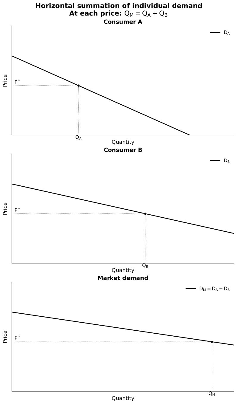
Caption: At the same reference price, Consumer A’s and Consumer B’s quantities are added horizontally to obtain market quantity demanded.

Types of demand

• Competitive demand: goods are substitutes, such as tea and coffee.
• Joint demand: goods are complements, such as printers and ink.
• Derived demand: demand for an input arises from demand for the final product, such as labour for construction.

For substitutes, a rise in the price of one good increases demand for the other. For complements, a rise in the price of one good decreases demand for the other. Derived demand creates a causal link between a product market and a factor market.

Quantity demanded versus demand

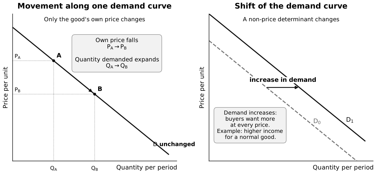
Caption: In the left panel, a fall in own price moves the market from A to B, down and right along an unchanged demand curve; the arrow shows expansion of quantity demanded, not a leftward curve shift. In the right panel, higher income for a normal good is one possible non-price cause of an increase in demand: the entire curve shifts right because buyers want more at every price. A fall in preference, a lower substitute price, or a higher complement price could instead shift demand left.

• Change in the good’s own price → change in quantity demanded → movement along demand.
• Change in another determinant → change in demand → curve shifts.

Do not confuse a downward-sloping demand curve with the statement “higher demand raises market price.” The curve’s negative slope describes a movement along one fixed demand schedule. “Higher demand” means the whole schedule shifts right. At the old price this creates a shortage; price then rises, producing a contraction along the new demand curve and an expansion along supply until a new equilibrium is reached.

Demand determinants

Determinant	Typical reasoning
Income	Normal-good demand rises with income; inferior-good demand falls
Price of a substitute	Higher substitute price raises demand for this good
Price of a complement	Higher complement price lowers demand for this good
Tastes and advertising	Greater preference raises willingness to buy
Population and demographics	More relevant consumers raise market demand
Expectations	Expected future price or income changes can alter current demand
Credit conditions	Easier borrowing can raise demand for credit-financed goods
Government policy or regulation	Eligibility rules, bans or mandated standards can change willingness or ability to buy
Exchange rates	For an export market, an appreciation can raise the foreign-currency price at a given domestic price and reduce foreign demand; always state the market and transmission clearly

Do not state a memorised direction without identifying the relationship. An income rise reduces demand only if the good is inferior.

Supply

Supply is the quantities of a good or service producers are willing and able to sell at different prices over a given period, ceteris paribus.

The law of supply states that price and quantity supplied are directly related, ceteris paribus.

Enrichment: why the supply curve slopes upward

Marginal-cost language is a useful bridge to Theme 2.2. Theme 2.1 questions mainly require you to distinguish movements from shifts and apply supply determinants accurately.

Why might supply slope upward?

• a higher output price makes units with higher marginal cost commercially worthwhile;
• existing producers have an incentive to expand quantity supplied using available capacity;
• diminishing marginal returns or increasingly costly inputs can raise the marginal cost of additional output.

Entry of new firms is better treated as a non-price increase in market supply, not as a movement along a fixed market-supply curve.

Quantity supplied versus supply

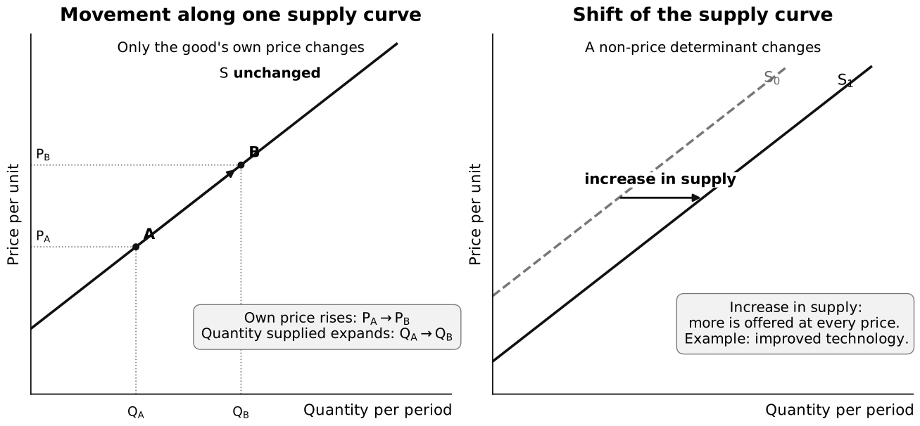
Caption: In the left panel, a rise in own price moves from A to B, up and right along an unchanged supply curve, so quantity supplied expands. In the right panel, better technology is one possible cause of an increase in supply: sellers can offer more at every price, so the entire curve shifts right. Higher input prices, a per-unit tax, or adverse weather could instead shift supply left.

• Change in the good’s own price → change in quantity supplied.
• Change in another determinant → change in supply.

Individual and market supply

Market supply is the horizontal sum of individual producers’ supply. At each price, add the quantities every producer is willing and able to sell:

$$Q_S(P)=\sum _{j=1}^m{Q}_{s,j}(P)$$

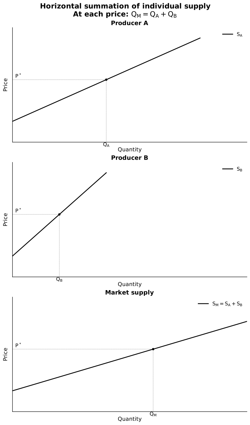
Caption: Producer A’s and Producer B’s quantities supplied at the same reference price are added horizontally to obtain market supply.

Supply determinants

Determinant	Typical reasoning
Input prices	Higher costs reduce profitability at each output price, decreasing supply
Technology/productivity	Lower unit cost increases supply
Taxes and subsidies	A per-unit tax raises marginal cost; a subsidy lowers it
Number of firms	Entry increases market supply; exit decreases it
Expectations	Expected future prices can alter current release of stocks
Natural conditions	Weather strongly affects agricultural supply
Regulation	Compliance costs or legal limits can reduce supply
Exchange rates	A depreciation may raise the domestic-currency cost of imported inputs and reduce supply, ceteris paribus

Related goods in production

• Competitive supply: resources can switch between goods. A higher price of palm oil may reduce rubber supply.
• Joint supply: producing one good also produces another. More beef production may increase hide supply.

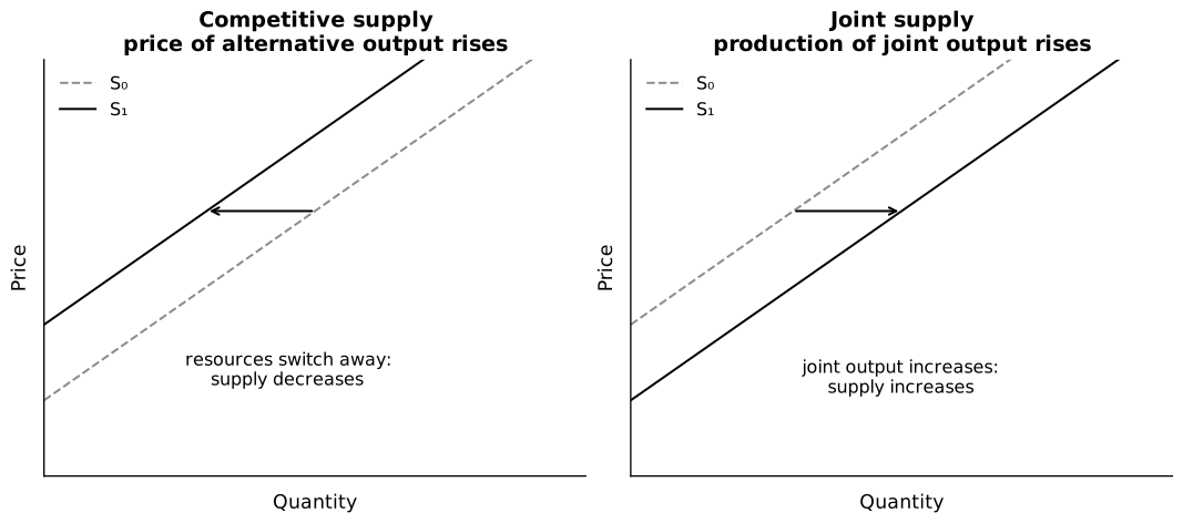
Caption: A more attractive alternative output draws shared resources away and decreases supply, while greater joint production increases supply of the accompanying output.

Keep the causal direction explicit. If palm oil and rubber compete for the same land, a rise in the price of palm oil raises its quantity supplied and encourages resource reallocation towards palm oil, thereby decreasing the supply of rubber. For joint products, greater production of one output mechanically makes more of the accompanying output available.

A disciplined shift explanation

Use this sequence:

1. Name the determinant.
2. Explain how it changes willingness or ability to buy/sell at each price.
3. State increase or decrease in demand/supply.
4. State the direction of the curve shift.
5. Only then combine it with the other curve to derive equilibrium effects.

Example:

An improvement in production technology raises output per unit of input, lowering unit cost. Producers are willing and able to supply more corn at every price, so supply increases and shifts right.

Ceteris paribus

Ceteris paribus means other relevant influences are held constant. It lets the model isolate one causal change. In real markets several determinants can change together, so the conclusion may require a simultaneous-shift analysis.

What is determined inside the model?

In a basic competitive-market diagram:

Type of quantity	Examples	Role in the model
Underlying conditions treated as given for the analysis	income, tastes, input prices, technology, number of firms, regulation	changes in these conditions shift demand or supply
Variables determined by market interaction	equilibrium price $P_e$ and equilibrium quantity $Q_e$	the intersection of demand and supply determines both together
Externally imposed constraint	a statutory ceiling, floor or quota	prevents or modifies the free-market outcome

The same variable can play different roles in different questions. For example, the good’s own price is a coordinate used to construct a demand schedule; in a free market its equilibrium value emerges from both demand and supply; under a binding price control its legal value is imposed by government. Always state which model is being used.

Required labour-market transfer

The same distinctions apply when labour is the good being traded:

• wage is the price of labour;
• a wage change causes movements along labour demand and labour supply;
• stronger demand for the final product increases the derived demand for labour and shifts labour demand right;
• migration, demographics, qualifications, participation decisions and non-wage working conditions can shift labour supply.

Syllabus boundary

Theme 2.1 requires labour-market application, but Marginal Revenue Productivity theory is not required.

Difficult distinctions

• A fall in price does not shift demand.
• “Demanded” is not the same as “demand.”
• A movement along one curve can occur because the other curve shifted.
• A producer’s cost change shifts supply; it does not directly shift demand.
• A labour-market wage is the price of labour, so a wage change causes movement along labour demand or supply.
• A rise in product demand can shift labour demand; it does not automatically shift labour supply.

Common pitfalls

• Omitting willing and able.
• Omitting the time period and ceteris paribus condition.
• Giving a list of determinants without causal reasoning.
• Treating a substitute as a complement.
• Confusing competitive supply with competitive demand.
• Drawing arrows that do not match the written direction.

Check your understanding

1. Explain how a rise in the price of coffee affects demand for tea.
2. Explain how a rise in energy prices affects the supply of aluminium.
3. Distinguish an increase in supply from an increase in quantity supplied.

Return to Price Mechanism and its Applications.