Elasticity Concepts and Applications

Elasticity as responsiveness

Elasticity compares the percentage response of one variable with the percentage change in a stated driver, ceteris paribus. Because it is a ratio of percentages, it has no unit and allows comparison across goods measured in different units.

Symbols used in this note

Symbol	Meaning
$\%\Delta$	percentage change; $\Delta$ means “change in”
$Q_d$	quantity demanded of the good per stated period
$Q_s$	quantity supplied of the good per stated period
$P$	the good’s own price
$Y$	consumer income
$Q_{d,A}$	quantity demanded of good A
$P_B$	price of a related good B

Read each formula as response divided by driver:

Elasticity	Responding variable (numerator)	Stated driver (denominator)
PED	$Q_d$	own price $P$
YED	$Q_d$	income $Y$
XED of A with respect to B	$Q_{d,A}$	price $P_B$
PES	$Q_s$	own price $P$

This language does not imply that only one factor ever affects demand or supply. It means the model isolates the stated driver while holding other relevant determinants constant.

Use the initial-value convention unless a question specifies the midpoint method:

$$\%\text{ change}=\frac{\text{change}}{\text{original value}}\times 100$$

State the base used. Initial-value percentages can differ depending on the direction of comparison; the midpoint method avoids that asymmetry when a question requests it.

Price elasticity of demand

$$PED=\frac{\%\Delta Q_d}{\%\Delta P}$$

PED is normally negative because price and quantity demanded move in opposite directions. Classification commonly uses the magnitude $|PED|$.

Magnitude	Classification	Interpretation
$|PED|>1$	price elastic	$Q_d$ changes more than proportionately
$0<|PED|<1$	price inelastic	$Q_d$ changes less than proportionately
$|PED|=1$	unit elastic	$Q_d$ changes in the same proportion
$PED=0$	perfectly inelastic	$Q_d$ does not respond to price
$|PED|\to \infty$	perfectly elastic	at the given price, any price rise reduces quantity demanded to zero, while a price fall makes demand unbounded in the idealised case

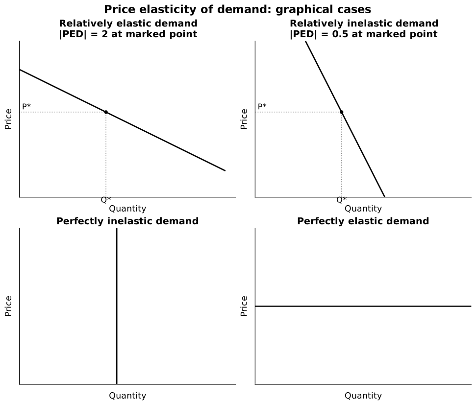
Caption: PED cases generated from explicit functions; the flatter-looking line is not automatically more elastic unless axes, units and comparison point are controlled. The numerical marked-point values illustrate the optional point-elasticity extension; the elasticity classifications themselves are core.

Determinants of PED

• more and closer substitutes → more elastic;
• necessity → more inelastic; luxury → more elastic;
• narrowly defined market → more elastic;
• smaller budget share → more inelastic;
• more time to adjust → more elastic;
• stronger habit or brand loyalty → more inelastic.

PED along a straight demand curve

PED varies along a linear demand curve:

• upper section: price is high and quantity is low, so demand is elastic;
• midpoint: unit elastic;
• lower section: price is low and quantity is high, so demand is inelastic.

Constant slope does not mean constant elasticity.

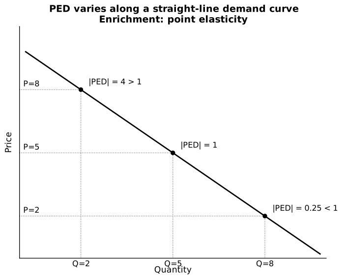
Caption: For the explicit line $P=10-Q$, point PED falls from elastic to unit elastic to inelastic as price falls and quantity rises, even though slope is constant.

Useful extension: point elasticity

For a differentiable demand curve, point PED can be written as

$$PED=\frac{d{Q}_d}{dP}\times \frac{P}{Q_d}.$$

This explains why identical slope does not imply identical elasticity at different points. Use the percentage formula unless a question or teacher specifically asks for point elasticity.

PED and total revenue

In an ordinary market without a tax/subsidy wedge, consumer expenditure on the good equals producer total revenue:

$$CE=TR=P\times Q$$

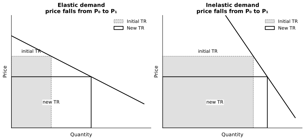
Caption: When price falls, the quantity response dominates for elastic demand but the price effect dominates for inelastic demand.

PED	Price rises	Price falls
Elastic	TR falls	TR rises
Inelastic	TR rises	TR falls
Unit elastic	TR unchanged	TR unchanged

The table describes a movement along an unchanged demand curve. For a large discrete change, use the question’s required percentage convention and compare the two $P\times Q$ values directly; rounding or an initial-value calculation may not produce exact equality at a reported $PED=-1$. This relationship does not automatically predict profit because costs may change. Under a tax or subsidy, distinguish the price consumers pay from the price producers receive.

Income elasticity of demand

$$YED=\frac{\%\Delta Q_d}{\%\Delta Y}$$

YED	Classification
$YED<0$	inferior good
$YED=0$	quantity demanded is unresponsive to income over the stated range
$0<YED<1$	normal necessity
$YED=1$	unit income-elastic normal good
$YED>1$	normal luxury

Core syllabus and enrichment boundary

For 9570 Theme 2.1, prioritise the sign: $YED>0$ identifies a normal good and $YED<0$ an inferior good. The necessity/luxury subdivision using the magnitude of positive YED is taught in the anchor notes and is useful for application, but it is enrichment rather than an explicit syllabus classification.

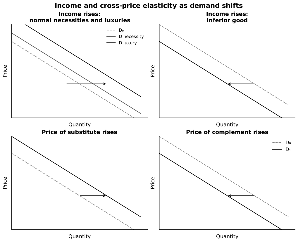
Caption: Income or related-good price changes are non-price demand determinants, so YED and XED applications involve shifts rather than movements along demand.

The sign classifies the good over the stated income range; the magnitude shows responsiveness.

YED depends on factors such as:

• whether the good is a necessity or luxury;
• the consumer’s existing income level;
• how broadly the product category is defined;
• the time available to adjust spending patterns.

Applications include forecasting demand during growth or recession, planning capacity and choosing a product portfolio. Classification can change across consumers, income levels, countries and time. “Luxury” is an elasticity classification, not a moral judgement.

Cross elasticity of demand

$$XE{D}_{A,B}=\frac{\%\Delta Q_{d,A}}{\%\Delta P_B}$$

XED	Relationship
$XED>0$	substitutes
$XED<0$	complements
$XED\approx 0$	weakly related or unrelated

The magnitude shows the strength of the relationship, although it depends on product definition, consumer group and time period. Firms use XED to identify close competitors, complementary products, pricing constraints and possible product bundles.

Be precise about direction: the denominator is the price change of B and the numerator is the demand change for A.

Price elasticity of supply

$$PES=\frac{\%\Delta Q_s}{\%\Delta P}$$

PES is normally non-negative:

PES	Classification	Interpretation
$PES=0$	perfectly price inelastic	quantity supplied does not respond
$0<PES<1$	price inelastic	quantity supplied changes less than proportionately
$PES=1$	unit elastic	quantity supplied changes in the same proportion
$PES>1$	price elastic	quantity supplied changes more than proportionately
$PES\to \infty$	perfectly elastic	suppliers offer output at one price in the idealised case

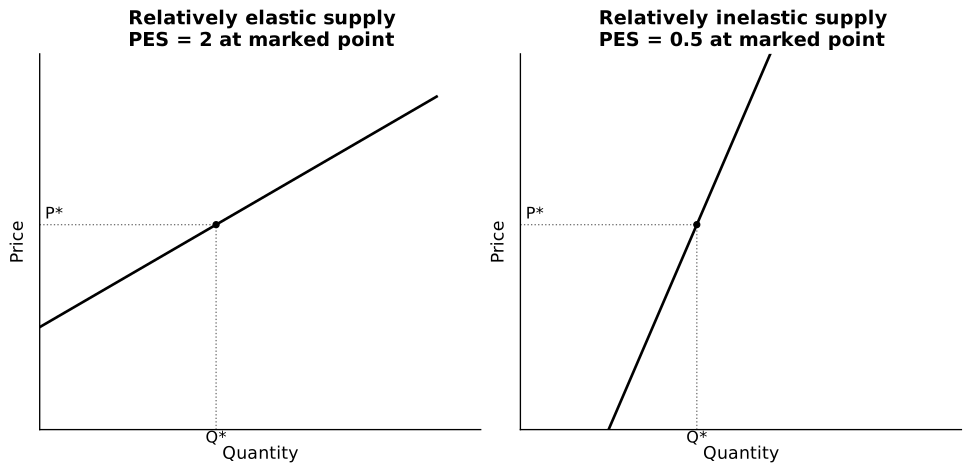
Caption: Supply is more elastic when quantity can respond strongly to price and more inelastic when production constraints limit adjustment. The marked-point values are calibrated illustrations; examination calculations should use the percentage-change formula unless another method is requested.

Determinants of PES

• time period;
• spare capacity;
• stocks of finished goods;
• ease of storing the product;
• mobility and availability of factors;
• production or gestation period.

Primary agricultural products often have inelastic short-run supply, while manufactured output may adjust more readily if stocks and spare capacity exist.

Time affects the ability to respond. Immediate supply may be fixed, while longer-run supply can be more elastic as firms vary capacity, train workers, enter or exit, and reorganise production.

Elasticity and market outcomes

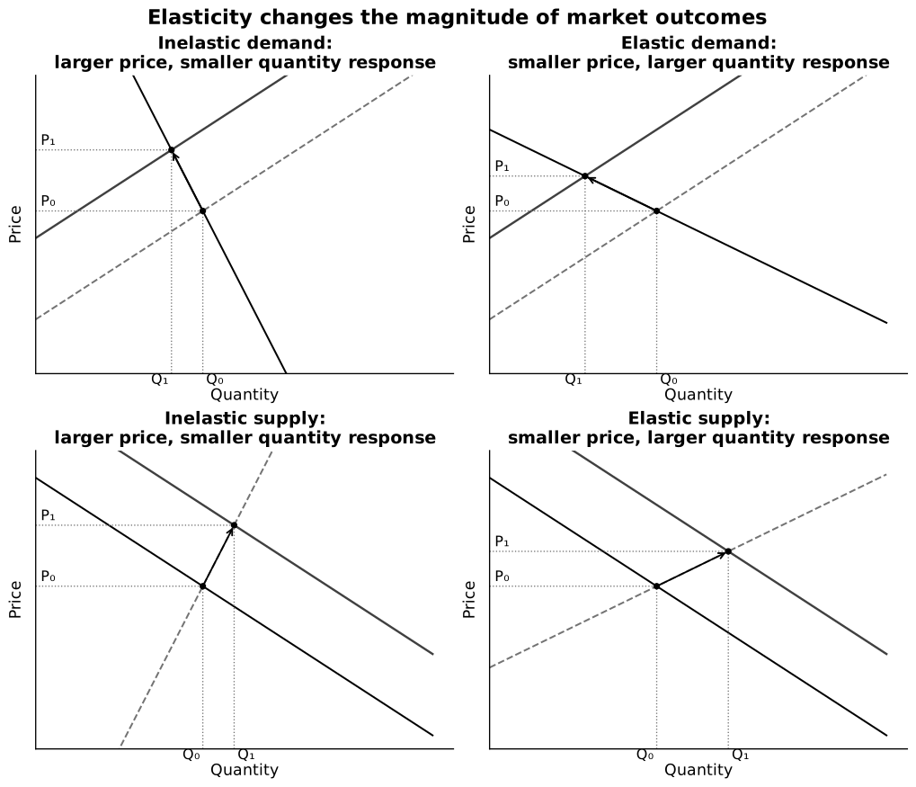
Caption: The calculated intersections demonstrate how relative curve responsiveness changes the split between price and quantity adjustment.

Applications:

• Inelastic supply makes demand shocks create larger price volatility.
• Inelastic demand makes supply shocks create larger price changes and smaller quantity changes.
• Relative PED and PES affect the changes in consumer and producer prices under a tax or subsidy.
• Tax revenue may be larger when demand is inelastic, other things equal.

Syllabus boundary

Formal knowledge of tax/subsidy incidence is not required in 9570 Theme 2.1. The elasticity insight above is retained as enrichment because it helps explain price changes, but do not treat incidence terminology as a compulsory learning outcome.

Worked calculations

PED

Price rises from 10 monetary units to 12 monetary units; quantity demanded falls from 100 to 70.

$$PED=\frac{-30/100\times 100}{2/10\times 100}=-1.5$$

Demand is price elastic using initial values. Total revenue falls from $10\times 100=1000$ to $12\times 70=840$, consistent with a price rise when demand is elastic.

YED

Income rises by 5% and demand rises by 8%.

$$YED=\frac{8\%}{5\%}=1.6$$

The good is a normal luxury over this range.

XED

The price of coffee rises by 10% and demand for tea rises by 4%.

$$XED=\frac{4\%}{10\%}=+0.4$$

Tea and coffee are substitutes, though not extremely close ones.

PES

Price rises from 20 monetary units to 25 monetary units; quantity supplied rises from 200 to 230.

$$PES=\frac{30/200\times 100}{5/20\times 100}=0.6$$

Supply is price inelastic over this range using initial values.

Limitations

Elasticity estimates may:

• rely on past data that no longer reflect preferences;
• change along a curve or across price ranges;
• change over time;
• be distorted by simultaneous determinant changes;
• differ between consumer groups and markets;
• guide revenue but not profit without cost information.

Common pitfalls

• Treating PED’s negative sign as “inelastic.”
• Using slope as elasticity.
• Dropping the sign of YED or XED.
• Calling every normal good a luxury; normal necessities have $0<YED<1$.
• Reversing the numerator and denominator.
• Treating an elasticity estimate as fixed forever.
• Predicting profit from PED alone.

Return to Price Mechanism and its Applications.