Government Intervention in Markets

Why intervene?

Possible objectives include:

• discourage or encourage consumption and production;
• raise government revenue;
• improve affordability;
• protect producer or worker income;
• stabilise prices;
• address efficiency or equity concerns.

The policy should be judged against its stated objective, opportunity cost and unintended effects.

For every intervention, distinguish:

• the legal rule or financial wedge;
• the new prices faced by consumers and producers;
• the quantity actually traded;
• effects on consumer expenditure and producer revenue;
• changes in consumer and producer surplus;
• government revenue or expenditure;
• implementation problems and alternatives.

Welfare scope boundary

Theme 2.1 explicitly requires changes in consumer and producer surplus. The accompanying total-surplus and deadweight-loss language is retained from the anchor notes as an enrichment bridge to Theme 2.3. Always state the benchmark assumptions before drawing a net-welfare conclusion.

Deadweight loss (DWL) is a fall in total surplus that is not received as a gain by consumers, producers or government. In the competitive no-externality benchmark, it usually represents mutually beneficial trades that no longer occur, or inefficient extra units for which marginal opportunity cost exceeds willingness to pay. A tax receipt or government saving is therefore not itself DWL: it is a transfer or fiscal effect that must be counted separately.

Indirect tax

A specific indirect tax is a fixed amount imposed per unit. It raises the marginal cost of supplying each unit, shifting supply vertically upward by the tax.

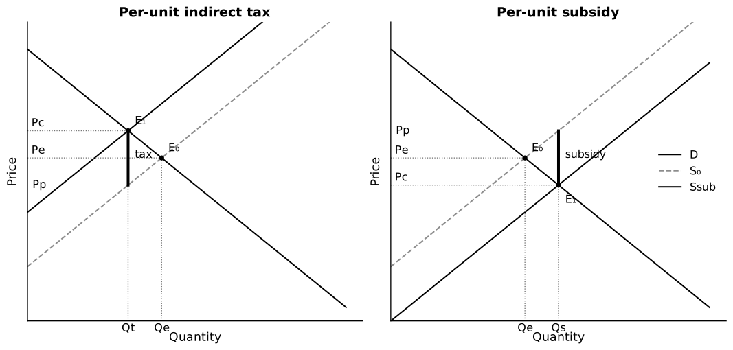
Caption: The function-based diagram compares the original and post-policy equilibria and shows the exact vertical tax or subsidy wedge between the consumer price $P_c$ and producer price $P_p$.

For a tax:

• consumer price rises from the original equilibrium;
• producer price after tax falls;
• equilibrium quantity falls;
• government revenue is collected on each unit sold;
• consumer and producer surplus usually fall;
• lost mutually beneficial trades create deadweight loss under the competitive benchmark.

Government revenue is:

$$\text{tax revenue}=\text{tax per unit}\times Q_{tax}.$$

Consumer expenditure $P_c{Q}_{tax}$ may rise or fall depending on PED because the consumer price rises while quantity falls. Producer revenue $P_p{Q}_{tax}$ falls in the standard diagram because both the net producer price and quantity sold fall.

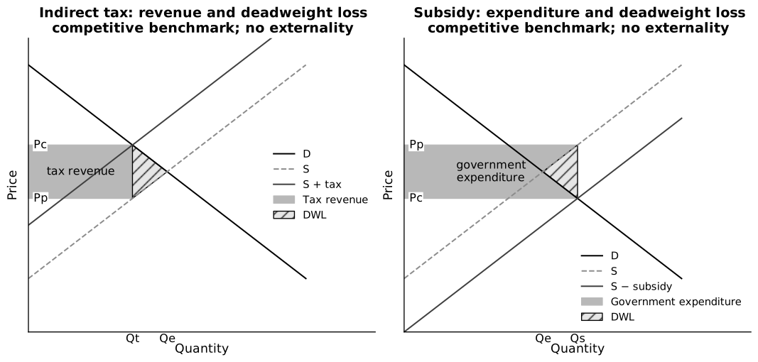
Caption: Under the stated competitive benchmark with no externality, each fiscal rectangle has height $|P_c-P_p|$ and the relevant post-policy quantity as its width; the hatched area is deadweight loss.

Enrichment bridge to Theme 2.3

Theme 2.1 requires effects on consumer and producer surplus. Netting those changes against government revenue or expenditure and identifying deadweight loss extends the analysis towards Theme 2.3. A corrective tax or subsidy may reduce an existing welfare loss, so the unqualified deadweight-loss result applies only to the no-externality competitive benchmark shown.

Enrichment: distribution of the tax wedge

Syllabus boundary

Formal knowledge of tax and subsidy incidence is not required in the 9570 syllabus. The following intuition is useful enrichment for explaining how elasticity affects market outcomes.

The legal obligation to remit a tax does not by itself determine how consumer and producer prices change.

• More inelastic demand relative to supply → consumers bear more.
• More inelastic supply relative to demand → producers bear more.

The less responsive side has fewer alternatives and tends to experience more of the price change associated with the wedge.

Evaluation

Effectiveness depends on:

• PED: inelastic demand means a smaller quantity reduction;
• availability of substitutes and evasion;
• size of the tax;
• administrative cost;
• distributional effects;
• whether tax revenue finances useful alternatives.

Subsidy

A per-unit subsidy lowers the marginal cost faced by producers, shifting supply vertically downward by the subsidy.

Effects:

• consumer price falls;
• producer price including subsidy rises;
• equilibrium quantity rises;
• government expenditure is incurred on each unit sold;
• consumer and producer surplus usually rise, but government expenditure and its opportunity cost must be included in welfare analysis.

Government expenditure is:

$$\text{subsidy expenditure}=\text{subsidy per unit}\times Q_{subsidy}.$$

Consumer expenditure $P_c{Q}_{subsidy}$ may rise or fall depending on PED because the consumer price falls while quantity rises. Producer revenue $P_p{Q}_{subsidy}$ rises in the standard diagram because both the gross producer price and quantity sold rise.

As enrichment, relative elasticity affects how the subsidy changes consumer and producer prices. Formal incidence terminology is not required.

Under the competitive benchmark with no external benefit, a subsidy can create overproduction: units beyond the original equilibrium have marginal cost above marginal willingness to pay. Subsidy evaluation should therefore consider targeting, additionality, fiscal sustainability, overconsumption and whether the policy corrects a genuine market problem.

Price ceiling

A price ceiling is the highest legal price.

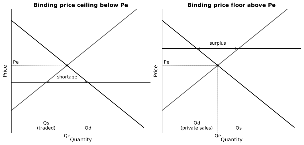
Caption: Only a ceiling below equilibrium or a floor above equilibrium is binding. The diagram distinguishes the shortage or surplus from actual private trades, which are constrained by $Q_s$ under the ceiling and $Q_d$ under the floor.

When a ceiling is binding:

• quantity demanded rises;
• quantity supplied falls;
• a shortage emerges.

Without government provision, actual legal transactions are constrained by the short side of the market, normally $Q_s$ at the controlled price. The numerical shortage is $Q_d-Q_s$; it is not the quantity traded.

Consumer expenditure and producer revenue on legal private-market sales are $P_{ceiling}{Q}_s$, which are lower than at the original equilibrium in the standard diagram because both price and quantity traded are lower. Producer surplus falls. Consumer surplus is ambiguous: successful buyers gain from the lower price, while excluded consumers lose trades and non-price rationing may impose extra costs. Total surplus falls under the competitive benchmark.

Possible intended outcome: greater affordability for consumers who obtain the product.

Possible unintended effects:

• queues and non-price rationing;
• black markets;
• lower quality;
• favouritism;
• reduced maintenance or investment;
• government expenditure if it purchases or provides additional supply.

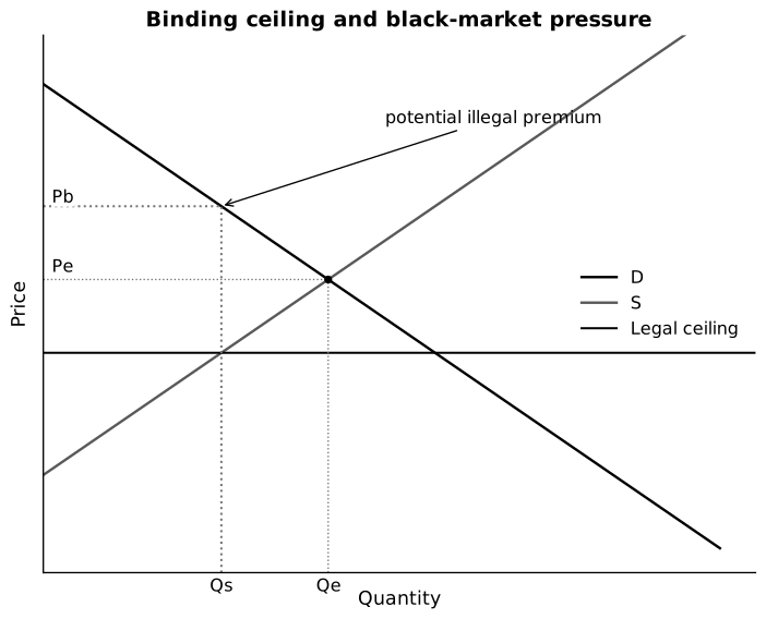
Caption: At the legally available quantity under a binding ceiling, consumers’ willingness to pay may exceed the controlled price, creating an illegal premium and black-market pressure.

A ceiling at or above equilibrium is non-binding.

Price floor

A price floor is the lowest legal price. Examples include agricultural support prices and minimum wages.

When a floor is binding:

• quantity supplied rises;
• quantity demanded falls;
• a surplus emerges.

Without government purchases, actual private-market transactions are constrained by demand, normally $Q_d$ at the controlled price. $Q_s-Q_d$ is excess supply, not automatically the quantity bought by government.

Private-market expenditure and producer revenue are $P_{floor}{Q}_d$; because price rises while private quantity sold falls, their direction depends on PED. Consumer surplus falls. Producer surplus may rise or fall depending on the elasticity of demand, the units actually sold and whether government purchases excess supply. Total surplus falls under the competitive benchmark unless another market problem justifies the intervention.

Possible effects:

• higher income for units still sold or workers still employed;
• unsold stocks or unemployment;
• government purchasing and storage cost;
• incentives for overproduction;
• evasion or movement into informal markets.

A floor at or below equilibrium is non-binding.

Production quota

A quota legally limits the quantity produced or supplied.

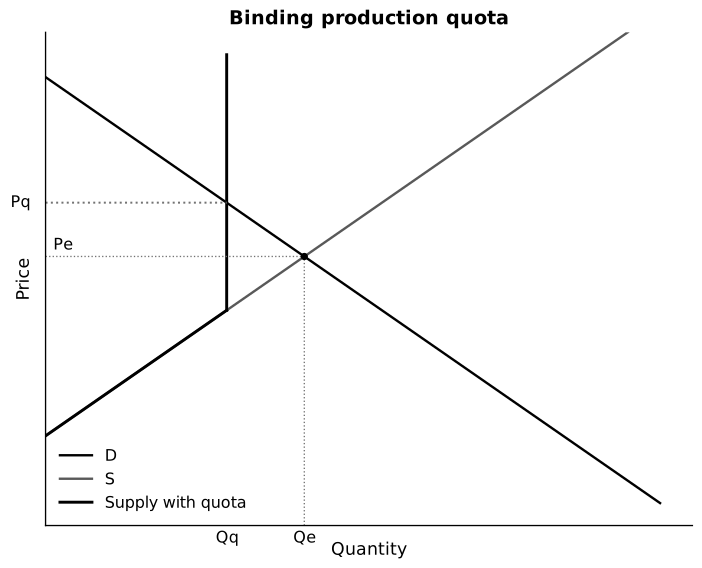
Caption: Effective supply follows the original supply curve up to $Q_q$ and then becomes vertical at the binding cap; the market-clearing price rises to the demand price at $Q_q$.

Possible purposes include limiting consumption, controlling congestion, protecting a resource or supporting producer income.

Effects of a binding quota below the free-market equilibrium quantity:

• quantity falls;
• market price rises;
• a scarcity or quota rent may emerge;
• allocation depends on how quota rights are distributed;
• deadweight loss may arise from forgone trades.

Because price rises while quantity falls, consumer expenditure and producer revenue may rise or fall depending on PED. Consumer surplus falls. The effect on producer surplus depends on the lost sales and whether producers receive quota rents; it should not be assumed to rise automatically.

If demand is more price inelastic, a given restrictive quota tends to cause a larger price increase. If producers can evade the rule or if imported/illegal substitutes are readily available, the quantity restriction may be less effective.

Evaluation:

• enforcement and monitoring;
• illegal supply or circumvention;
• fairness in allocating licences;
• rent-seeking;
• whether quota rights can be traded;
• administrative cost and policy alternatives.

Worked numerical map aligned with the figures

The intervention figures use the inverse curves:

$$P_D=10-Q,P_S=2+Q.$$

The free-market equilibrium is $Q_e=4$ and $P_e=6$.

• Tax of 2 per unit: taxed supply is $P=4+Q$, giving $Q_t=3$ and $P_c=7$. Producers retain $P_p=7-2=5$, so tax revenue is $2\times 3=6$.
• Subsidy of 2 per unit: the consumer-facing subsidised supply is $P=Q$, giving $Q_s=5$ and $P_c=5$. Producers receive $P_p=5+2=7$, so government expenditure is $2\times 5=10$.
• Ceiling at $P=4.5$: $Q_d=5.5$ and $Q_s=2.5$. The shortage is $3$, but legal quantity traded is normally $2.5$.
• Floor at $P=7.5$: $Q_d=2.5$ and $Q_s=5.5$. The surplus is $3$, but private sales are normally $2.5$ unless government purchases excess supply.
• Quota at $Q_q=2.8$: demand implies $P_q=7.2$. The original supply price at that quantity is $4.8$; the difference can become quota rent if quota holders capture it.

This numerical map reinforces three distinctions: a shortage or surplus is not the quantity traded, a tax or subsidy creates two relevant prices, and a quota rent depends on ownership of the quota right.

Welfare comparison

Policy	Price to consumers	Quantity	Fiscal effect	Common unintended effect
Tax	rises	falls	revenue	evasion or regressive burden
Subsidy	falls	rises	expenditure	fiscal cost or overuse
Price ceiling	legally lower	normally constrained by $Q_s$	possible expenditure	shortage/black market
Price floor	legally higher	normally constrained by $Q_d$	possible purchase cost	surplus/unemployment
Quota	usually rises	legally limited	possible licence revenue	quota rent/illegal supply

The table gives typical effects under standard assumptions. A control must be binding to alter the free-market outcome. Context and elasticity can change magnitudes and distribution.

Answer framework

1. State the policy and objective.
2. Establish initial equilibrium.
3. Show the intervention accurately.
4. Explain price and quantity adjustment.
5. Identify affected agents.
6. Analyse surplus, revenue/expenditure and unintended effects.
7. Evaluate using elasticity, time, enforcement, information, equity and alternatives.
8. Give a conditional judgement.

Common pitfalls

• Drawing tax as a demand shift without justification.
• Failing to distinguish consumer and producer prices.
• Measuring tax revenue using the original quantity.
• Treating a non-binding control as effective.
• Calling $Q_d-Q_s$ actual sales under a ceiling; actual legal sales are limited by the short side, normally $Q_s$.
• Assuming all producers benefit from a price floor.
• Treating excess supply under a floor as government purchases when no purchase scheme is stated.
• Ignoring fiscal opportunity cost.
• Presenting formal incidence terminology as compulsory syllabus content.
• Concluding from a diagram without discussing enforcement or elasticity.

Return to Price Mechanism and its Applications.