Market Equilibrium, Price Mechanism and Surplus

Equilibrium and disequilibrium

Market equilibrium occurs where:

$$Q_d=Q_s$$

There is no inherent pressure for price to change while other conditions remain unchanged. Equilibrium is not necessarily socially ideal; it is first a market-clearing condition.

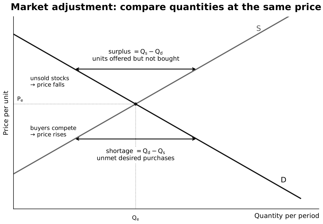
Caption: Compare $Q_d$ and $Q_s$ at the same stated price. Above equilibrium, excess supply is the horizontal distance $Q_s(P)-Q_d(P)$: units offered for sale but not bought. Below equilibrium, excess demand is $Q_d(P)-Q_s(P)$: desired purchases that cannot be satisfied. These are quantities of the same good per period, not triangular areas.

Price below equilibrium

$Q_d>Q_s$, so there is a shortage (excess demand):

$$\text{shortage at price }P=Q_d(P)-Q_s(P).$$

1. Consumers compete for limited units.
2. Sellers have an incentive to raise price.
3. Higher price contracts quantity demanded and expands quantity supplied.
4. The shortage narrows until $Q_d=Q_s$.

Price above equilibrium

$Q_s>Q_d$, so there is a market surplus (excess supply):

$$\text{surplus at price }P=Q_s(P)-Q_d(P).$$

Here, “surplus” means a physical excess quantity of the good offered during the period; it is different from consumer surplus or producer surplus, which are monetary measures of gains from trade.

1. Unsold stocks accumulate.
2. Sellers cut price to clear inventories.
3. Lower price expands quantity demanded and contracts quantity supplied.
4. The surplus narrows until equilibrium is restored.

The model assumes prices can adjust and that buyers and sellers respond to them. Contracts, menu costs, regulation or imperfect information can slow adjustment.

Analysing a market shock

Use this chain:

1. Define the market.
2. State the initial equilibrium.
3. Identify the determinant.
4. Explain which curve shifts and why.
5. Identify shortage or surplus at the old price.
6. Explain the direction of price adjustment.
7. Trace movements along the unshifted curve.
8. State the new equilibrium price and quantity.

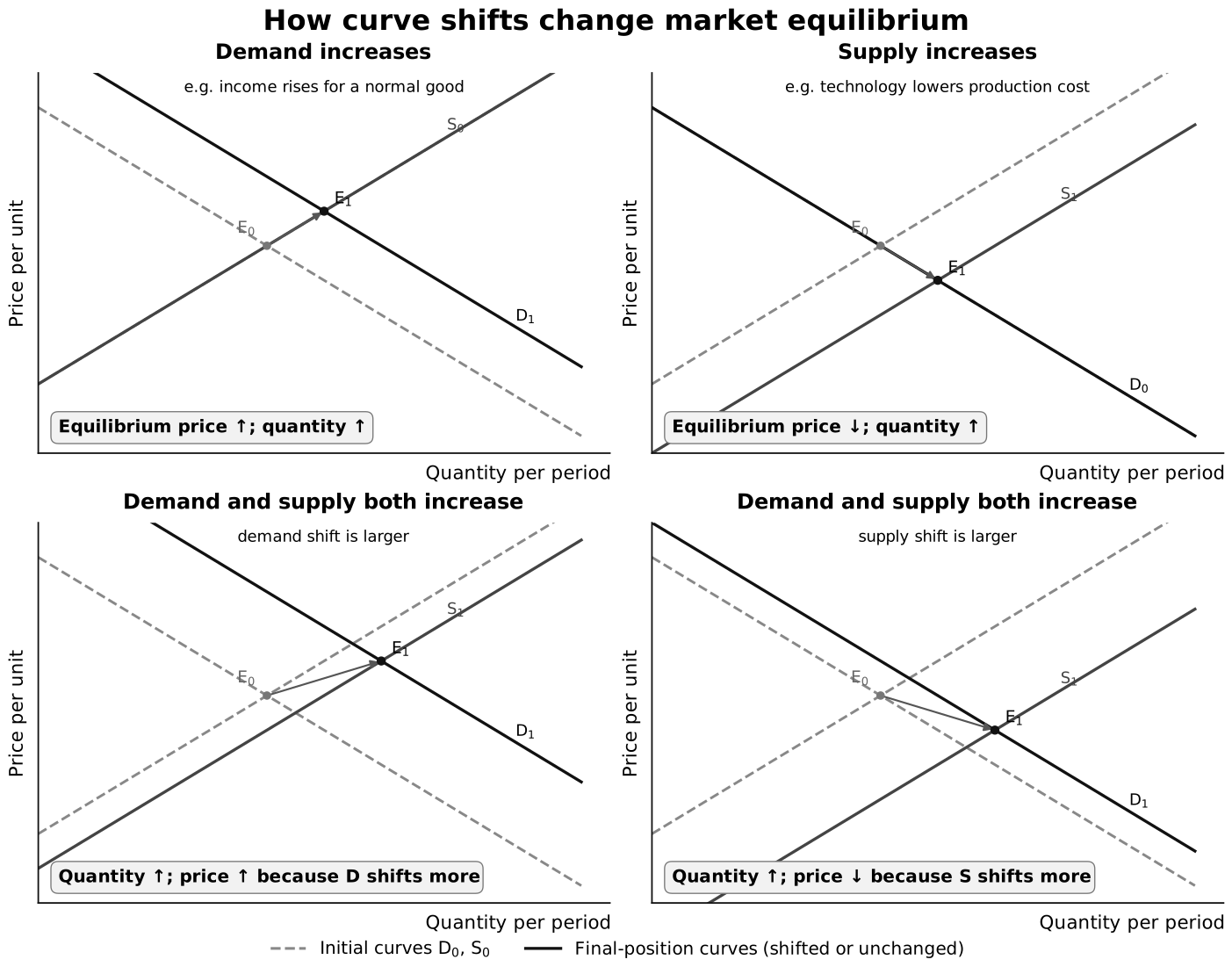
Caption: The upper-left panel shows higher income increasing demand for a normal good, raising equilibrium price and quantity. The upper-right panel shows lower production cost increasing supply, lowering equilibrium price and raising quantity. In the lower panels both curves increase, so equilibrium quantity rises; whether price rises or falls depends on which curve shifts farther.

The good’s own price is not listed as a shift determinant: a change in own price causes a movement along an existing curve. Income, tastes, related-good prices, technology and input costs are examples of non-price determinants that shift curves. In the free-market model, equilibrium $P_e$ and $Q_e$ are jointly determined after these schedules interact. Under a binding government control, the legal price is imposed and need not clear the market.

Single shifts

Change	Equilibrium price	Equilibrium quantity
Demand increases	rises	rises
Demand decreases	falls	falls
Supply increases	falls	rises
Supply decreases	rises	falls

Simultaneous shifts

When both curves shift, separate the effects:

• Demand and supply both increase: quantity rises, price is ambiguous.
• Demand and supply both decrease: quantity falls, price is ambiguous.
• Demand increases while supply decreases: price rises, quantity is ambiguous.
• Demand decreases while supply increases: price falls, quantity is ambiguous.

Resolve the ambiguous variable only if the relative shifts are known.

Worked equilibrium and demand-shift example

Suppose market demand and supply are:

$$Q_d=100-5P,Q_s=10P-20.$$

At equilibrium:

$$100-5P=10P-20\Rightarrow P_e=8,Q_e=60.$$

Now suppose demand increases to $Q_d^{\prime }=130-5P$, while supply is unchanged. At the old price $P=8$, quantity demanded is $90$ but quantity supplied is $60$, so a shortage of $30$ creates upward pressure on price. The new equilibrium is:

$$130-5P=10P-20\Rightarrow P_1=10,Q_1=80.$$

The example illustrates the complete reasoning chain: demand shifts right, a shortage appears at the old price, price rises, quantity supplied expands along the unchanged supply curve, and a new equilibrium is reached.

Expenditure, revenue and surplus after a market shift

The syllabus requires more than the new equilibrium price and quantity.

When consumers and producers face the same price:

$$\text{consumer expenditure}=\text{producer revenue}=P\times Q$$

After a shift:

1. determine the new equilibrium $P$ and $Q$;
2. compare the old and new rectangles $P\times Q$;
3. for a supply shift that moves the market along an unchanged demand curve, use PED to determine which of the opposing price and quantity effects dominates;
4. redraw consumer and producer surplus using the new equilibrium price and quantity.

For a single demand shift with unchanged supply, price and quantity move in the same direction. Hence an increase in demand raises $P\times Q$, while a decrease in demand lowers it. For a single supply shift, price and quantity move in opposite directions along unchanged demand, so PED is needed to determine the change in consumer expenditure and producer revenue.

Typical surplus reasoning under otherwise unchanged competitive conditions:

• an increase in demand usually raises producer surplus because price and quantity sold rise; the change in consumer surplus is not determined by the price rise alone because willingness to pay has also changed;
• an increase in supply usually raises consumer surplus because price falls and quantity traded rises; the change in producer surplus is not determined by the price fall alone because producers’ marginal costs have changed;
• a decrease in demand or supply reverses the relevant shift but still requires comparison of the complete old and new areas.

Do not use a one-line rule such as “higher price means lower consumer surplus” when the demand curve itself has shifted.

Price mechanism functions

Signalling

A price rise signals that demand has increased relative to supply or that the good has become more scarce.

Incentive

If a higher price is not fully offset by higher costs, the prospect of greater profitability encourages producers to expand output, enter or redirect resources towards the market.

Rationing

Price allocates limited output among competing buyers according to willingness and ability to pay.

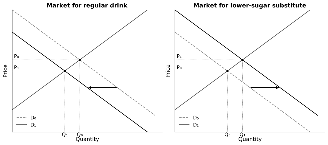
Caption: Preference changes lower the equilibrium price and quantity in one market while raising them in a substitute market, guiding resources toward the output consumers value more.

The complete chain is:

preferences change → demand shifts → disequilibrium at old prices → prices change → consumers and producers respond → resources move → new equilibria emerge.

The three functions jointly address the allocation questions:

• what to produce: resources move towards goods whose relative prices and expected profitability rise;
• how to produce: changing relative input prices encourage substitution towards lower-cost production methods;
• for whom to produce: output is rationed through prices and purchasing power.

This coordination is decentralised: no single agent needs to know every consumer preference or production condition.

Consumer surplus

For one traded unit, consumer surplus is the buyer’s maximum willingness to pay minus the price actually paid. The height of the demand curve at quantity $q$ represents marginal willingness to pay for that unit. Therefore, the vertical gap between demand and the transaction price measures consumer surplus on that unit.

Adding those non-negative vertical gaps over all units traded gives the area below demand and above the transaction-price line, up to the traded quantity. In a simple competitive equilibrium with a common market price, that line is $P_e$. The definition remains valid when the actual price is not the original equilibrium price.

For a triangular area bounded by linear curves:

$$CS=\frac{1}{2}\times \text{base}\times \text{height}$$

Producer surplus

For one traded unit, producer surplus is the price received minus the producer’s minimum acceptable price for supplying that unit. In the competitive benchmark, the height of supply at quantity $q$ represents the marginal opportunity cost, or the value of resources in their next-best use. The vertical gap between the transaction price and supply therefore measures producer surplus on that unit.

Adding these gaps over all units traded gives the area above supply and below the transaction-price line. At a simple competitive equilibrium, buyers pay and sellers receive $P_e$. Under a tax, however, consumer surplus is assessed using the consumer price $P_c$ while producer surplus is assessed using the producer price $P_p$.

$$PS=\frac{1}{2}\times \text{base}\times \text{height}$$

for a triangular producer-surplus area.

Producer surplus differs from:

• revenue, which is $P\times Q$;
• profit, which subtracts both variable and fixed costs.

Total surplus and efficiency

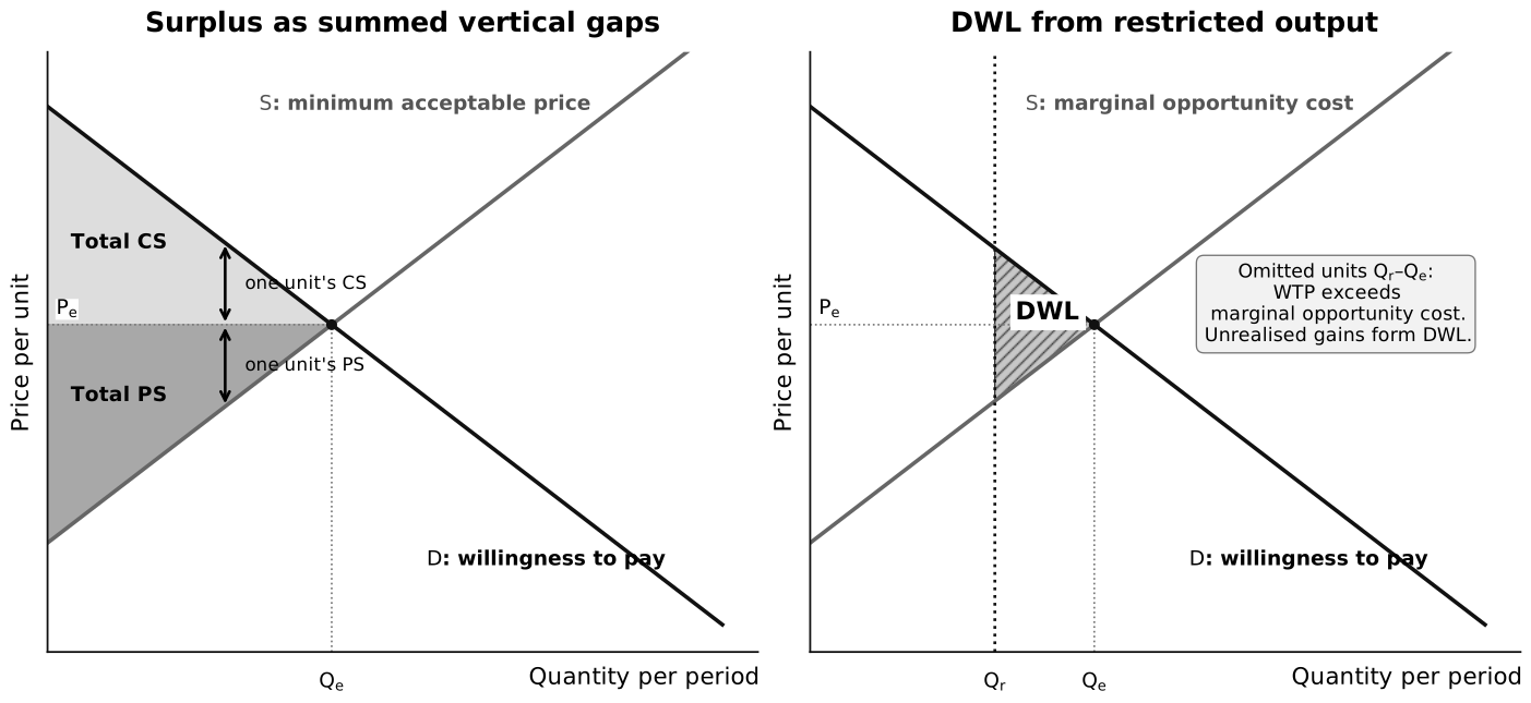
Caption: In the left panel, each short vertical gap above $P_e$ is consumer surplus on one unit and each gap below $P_e$ is producer surplus on one unit; summing the gaps creates the shaded areas. In the right panel, restricting output to $Q_r$ prevents trades between $Q_r$ and $Q_e$ even though willingness to pay exceeds marginal opportunity cost. The hatched sum of these unrealised gains is deadweight loss.

Why do these shapes represent surplus?

The areas are not arbitrary decorations. Imagine dividing quantity into many thin units of width $\Delta q$:

• consumer gain on one thin unit is approximately $[P_D(q)-P_{paid}]\Delta q$;
• producer gain on one thin unit is approximately $[P_{received}-P_S(q)]\Delta q$.

Adding the thin strips gives the shaded areas. With straight curves and one horizontal equilibrium price, the boundaries happen to form triangles. With curved schedules or different transaction prices, the shapes need not be triangular.

The dark-grey region in the figure is not consumer surplus merely because it lies below demand. Consumer surplus must lie above the price paid and below demand. Producer surplus lies below the price received and above supply. The market-price line separates the two per-unit gains.

Mathematical interpretation (enrichment)

For continuous inverse curves $P_D(q)$ and $P_S(q)$ at a common equilibrium price $P_e$,

$$CS={\int }_0^{Q_e}[P_D(q)-P_e]dq,PS={\int }_0^{Q_e}[P_e-P_S(q)]dq.$$

The integral is simply a compact way to add all the thin vertical surplus strips.

Deadweight loss

Deadweight loss (DWL) is total surplus that disappears rather than being transferred to another party. In the output-restriction example, units between $Q_r$ and $Q_e$ are not traded even though buyers’ willingness to pay exceeds sellers’ marginal opportunity cost. Every omitted unit therefore had a positive potential net gain. Adding those unrealised vertical gaps gives the hatched DWL area.

For the illustrated restriction:

$$DWL={\int }_{Q_r}^{Q_e}[P_D(q)-P_S(q)]dq.$$

With straight curves, the gap narrows to zero at $Q_e$, so the DWL is triangular. This benchmark assumes competitive markets, no externalities and prices that reflect opportunity costs; later market-failure analysis may change the relevant social-benefit or social-cost curves.

At competitive equilibrium, under the stated benchmark assumptions:

• marginal willingness to pay equals marginal opportunity cost;
• every mutually beneficial unit is traded;
• $CS+PS$ is maximised.

This conclusion relies on assumptions such as:

• no external costs or benefits;
• adequate information;
• competitive behaviour;
• prices reflecting relevant opportunity costs;
• no equity objective beyond total surplus.

It therefore does not prove that every unregulated market outcome is socially desirable.

Bridge to Theme 2.3

The total-surplus benchmark prepares you for market failure. Externalities, imperfect information, market power or equity concerns can make the free-market outcome socially undesirable even though the market clears.

Applications

Labour market

Demand for labour is derived from demand for final output. Wage is the price of labour, and employment is the equilibrium quantity.

For example:

stronger demand for healthcare services → greater derived demand for nurses → labour-demand curve shifts right → shortage of nurses at the original wage → upward pressure on wages and an expansion of labour supplied → higher equilibrium wage and employment, ceteris paribus.

Labour supply may shift because of migration, population structure, qualifications, participation decisions or non-wage working conditions. Institutional features such as contracts, collective bargaining and minimum wages may prevent immediate market clearing.

Syllabus boundary

Labour-market application is required. Marginal Revenue Productivity theory is not required.

Foreign-exchange market

Demand for SGD can rise when foreigners buy more Singapore exports or assets. Other things equal, the SGD appreciates under a market exchange-rate system.

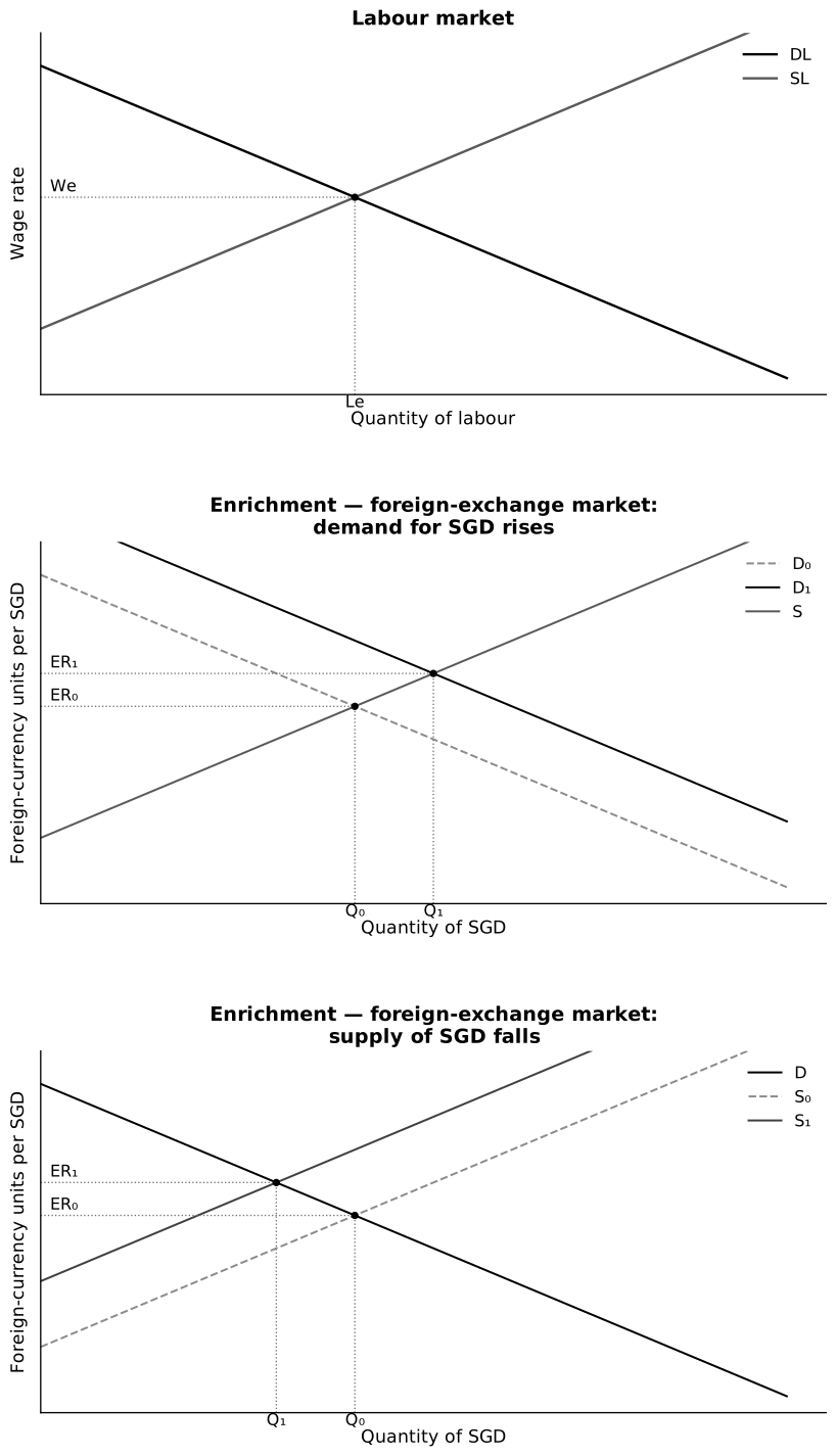
Caption: The same equilibrium method applies after relabelling the axes. In the enrichment panels the exchange rate is foreign-currency units per SGD, so stronger demand for SGD or reduced supply of SGD raises this rate and represents appreciation, ceteris paribus.

Enrichment

The foreign-exchange example is a useful transfer of the model. The syllabus explicitly names the labour market, so prioritise labour-market application for Theme 2.1 revision.

Evaluation

The speed and quality of adjustment depend on:

• PED and PES;
• information and expectations;
• stocks and spare capacity;
• entry barriers;
• government controls;
• time period;
• bargaining power and competition.

Common pitfalls

• Saying “shortage shifts demand.”
• Jumping from a determinant to the final outcome without adjustment.
• Assuming both price and quantity must be ambiguous under simultaneous shifts.
• Treating willingness to pay as identical to social benefit.
• Calling producer surplus profit.
• Assuming the direction of consumer expenditure or producer revenue from price alone when quantity also changes.
• Assuming a shift in demand has the same consumer-surplus effect as a movement along an unchanged demand curve.
• Applying a product-market determinant mechanically to labour or currency markets.

Return to Price Mechanism and its Applications.